Cloth Simulation

Part I: Masses and Springs

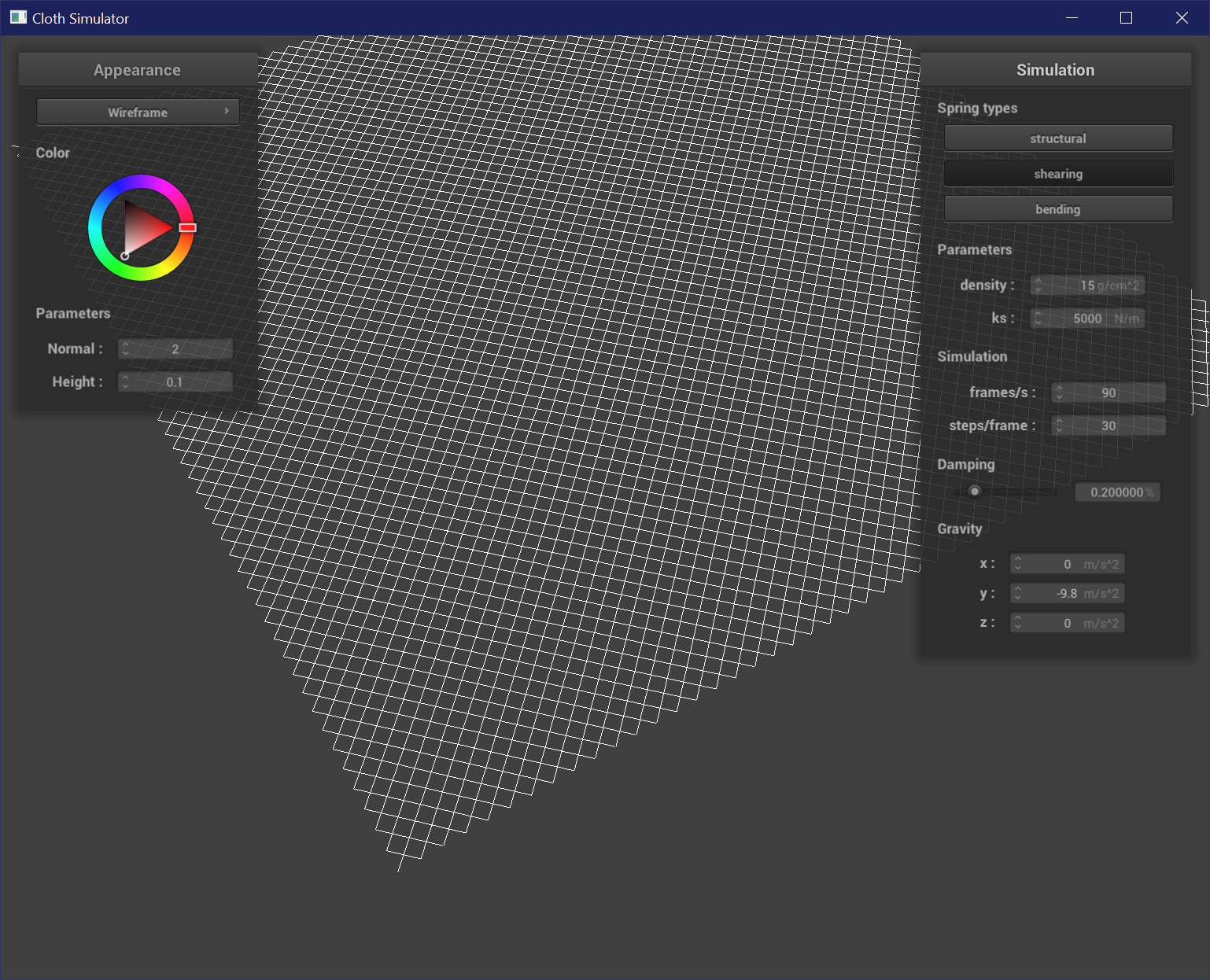
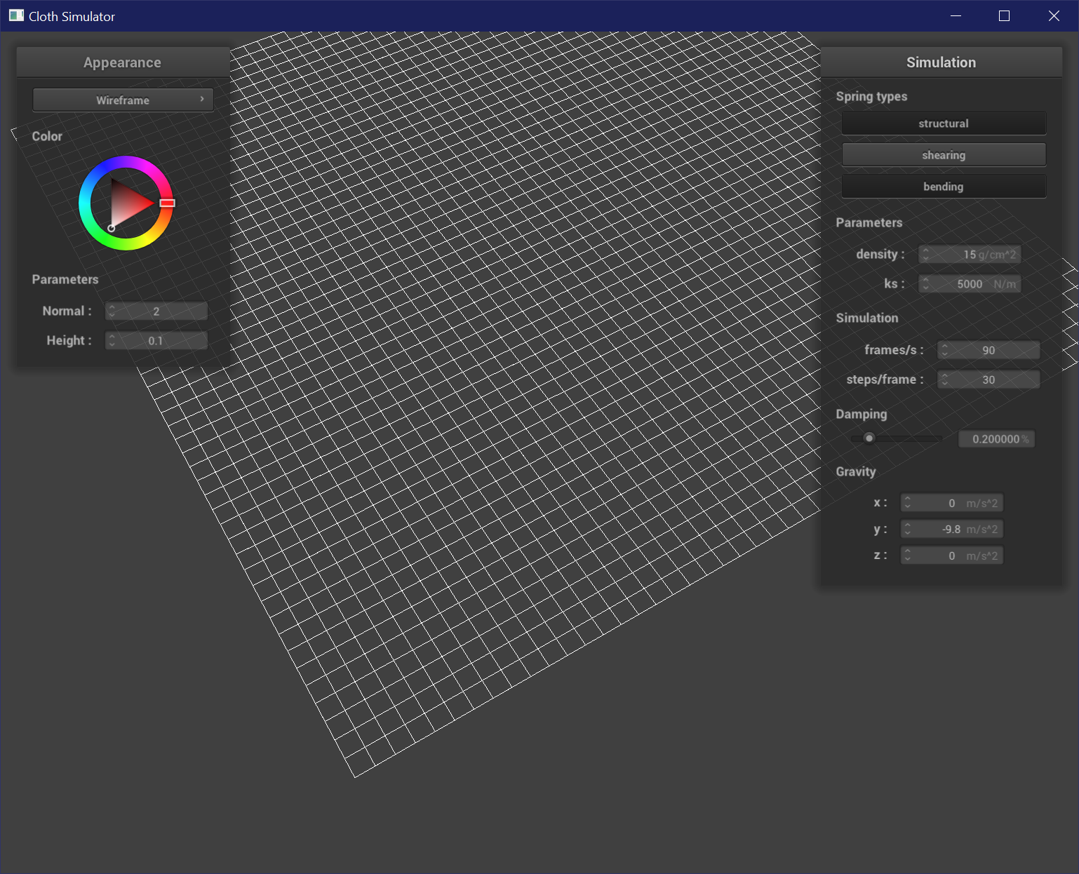
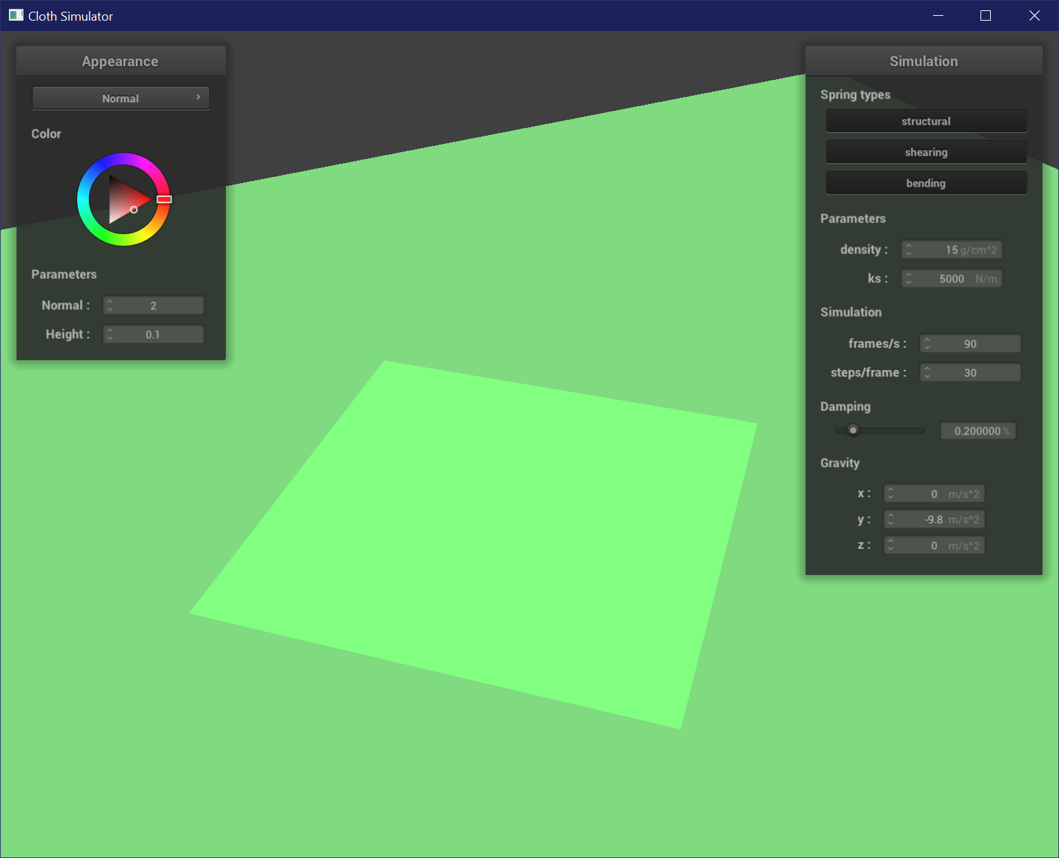
To set up the cloth wireframe, I spread out num_width_points x num_height_points evenly in a width x height rectangle. If the cloth is oriented in the horizontal direction, then I set the y-coordinate of each of the points to 1.0. If the cloth is oriented in the vertical direction, then I set the z-coordinate of each of the points to a small offset randomly generated between -1/1000 and 1/1000. If any of the points are considered pinned, then I set a boolean flag on that point.

Now that all of the points are set, I need to generate springs between each of the points to define the cloth's behaviors. There are three kinds of springs:
Structural: links a point to a point above and a point to the left.
Shearing: links a point to a point in the upper left and a point in the upper right.
Bending: links a point to a point two above and a point two right.

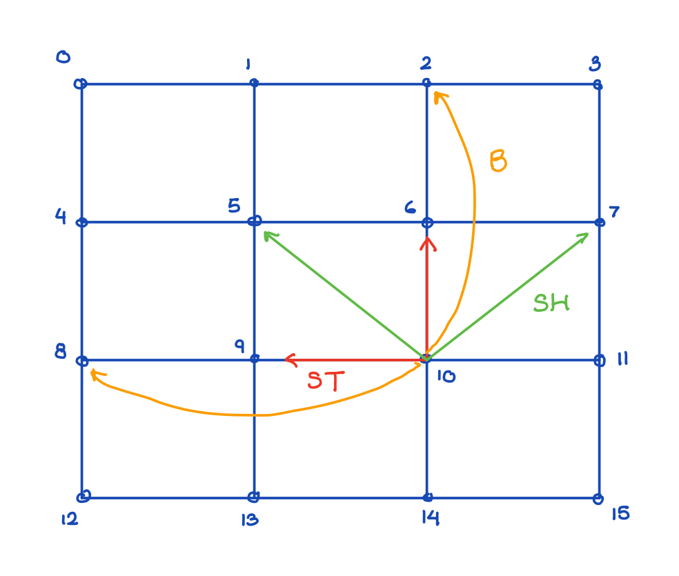
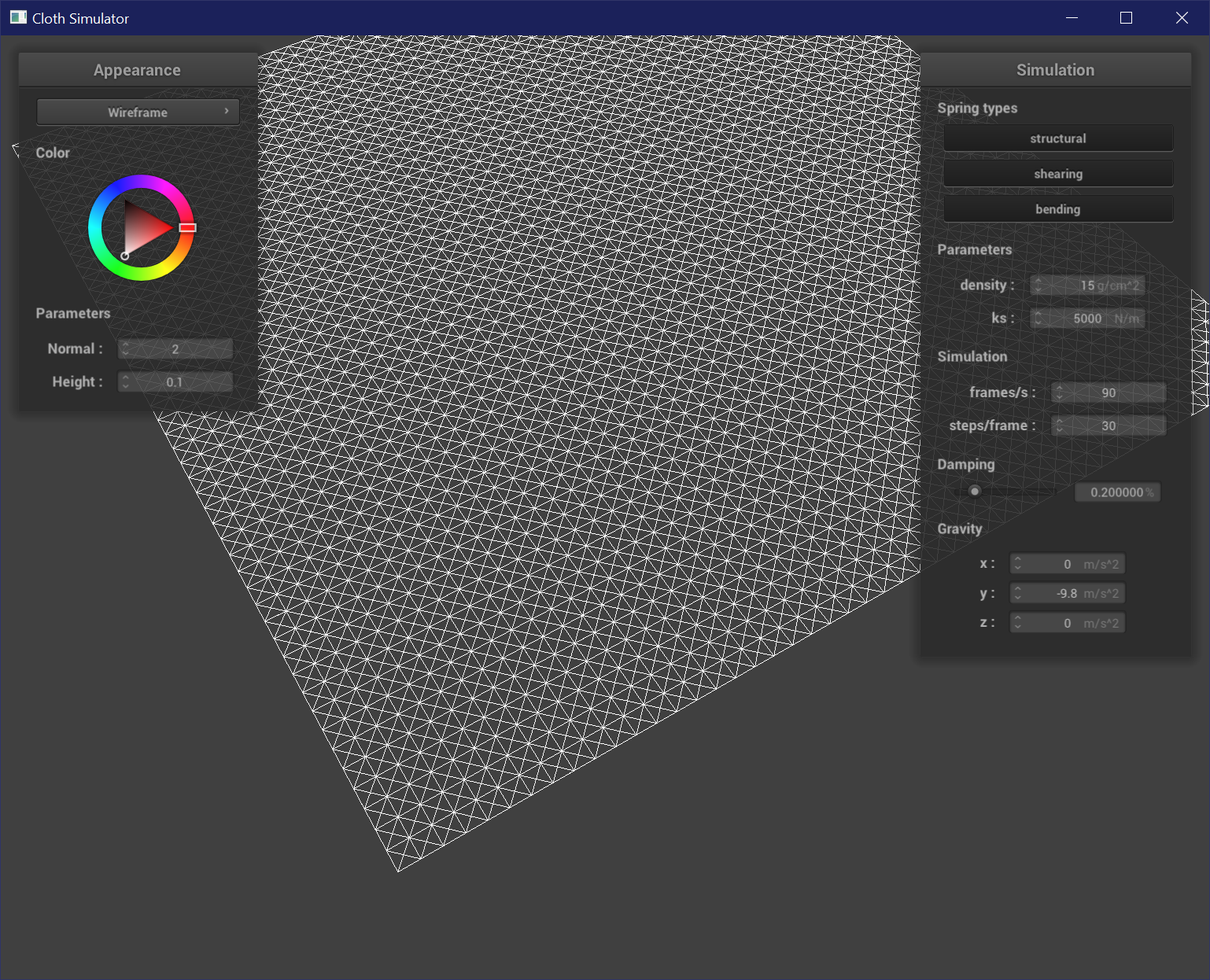
Notice how the shear springs are generated diagonally, and structural and bending springs are generated vertically and horizontally.

Part II: Simulation Via Numerical Integration

To simulate how cloth pulls and drags at pinned points, I used Hooke's Law as well as Newton's 2nd law to simulate the forces applied to different point masses. All points were effected by external forces such as gravity calculated by F = ma. Then, for each spring, the force applied to the two points connecting a spring are subject to correctional forces defined by Hooke's Law, calculated as F_s = k_s * (||p_a - p_b|| - l). This force is a magnitude, so to apply the forces to the points it needs to be multiplied by a vector with in the direction of point a. If the spring currently iterated on is a bending spring, the spring constant is multiplied by 0.2 to reduce its strength.

Now that the forces for each point mass have been calculated, I need to apply the change in position relative to the acceleration from the calculated forces. I used an approximation of Verlet integration, x_t+dt = x_t + (1 - d) * (x_t - x_t-dt) + a_t * dt^2, where a_t is found from F = ma. Each timestep is updated according to Verlet integration so long as the point mass is not pinned.

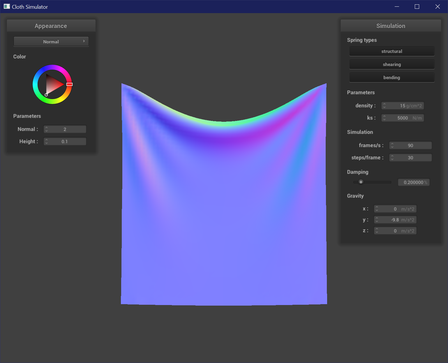
To prevent points from over-correcting or moving too far apart, I constrainted all points to be within 110% of the resting length.

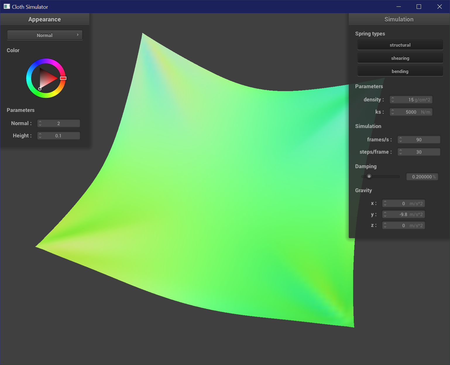
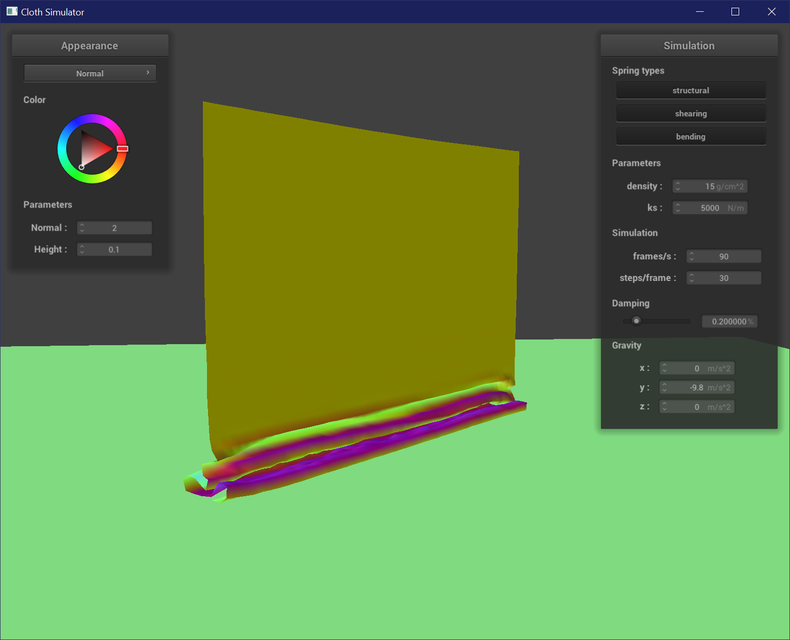
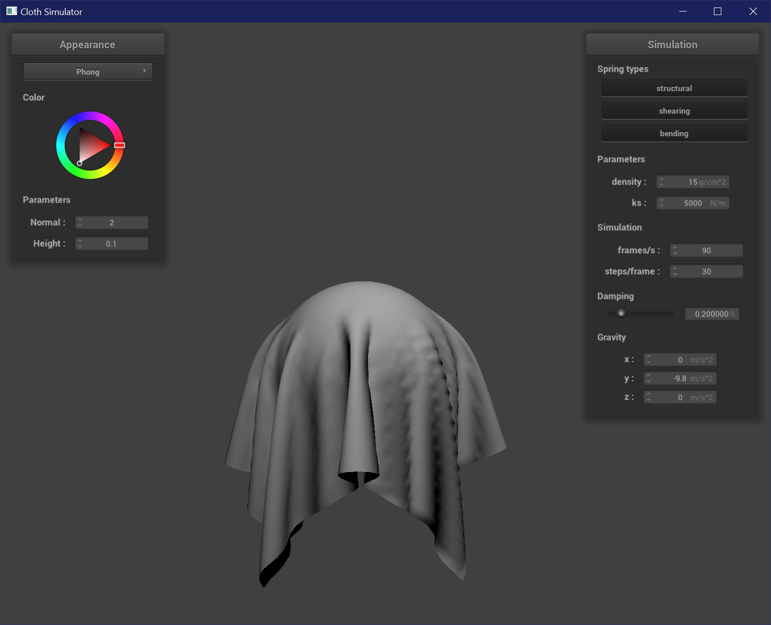
Once all of the above is set, the cloth falls nicely from pinned points, pulling taut at the corners and forming folds or wrinkles.

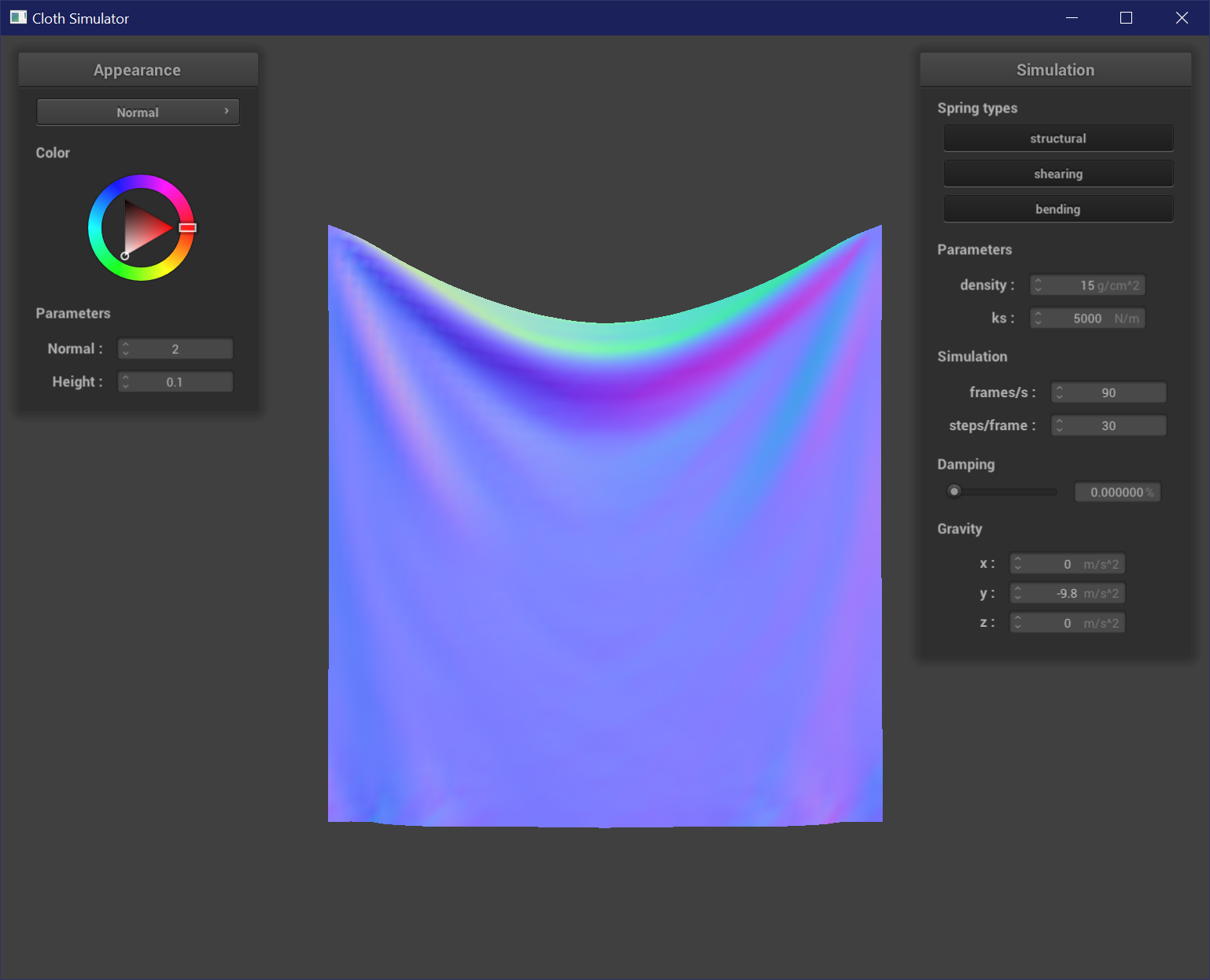
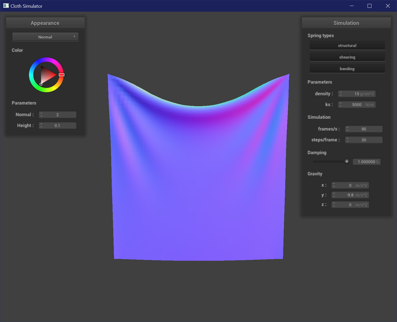
Varying Damping

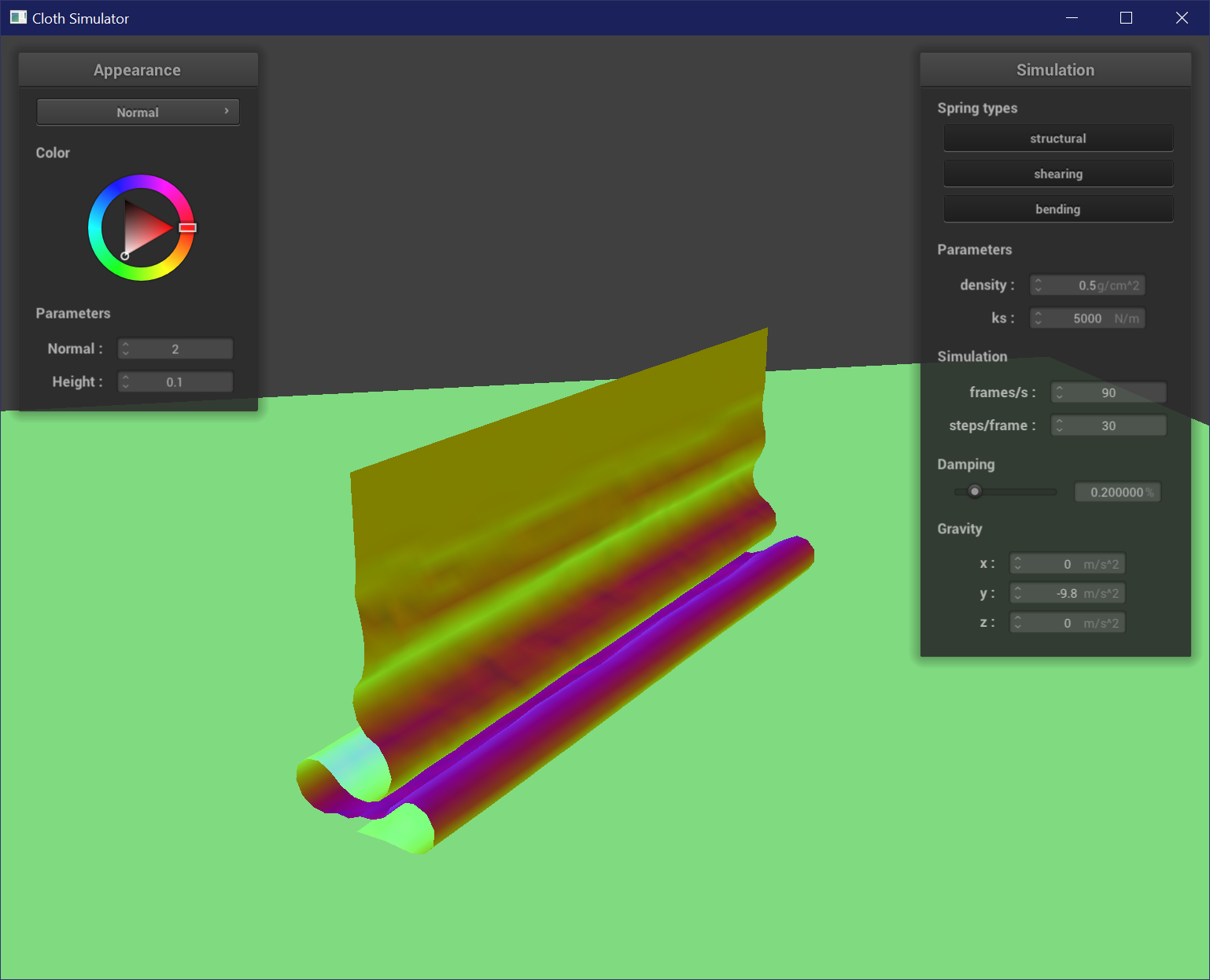
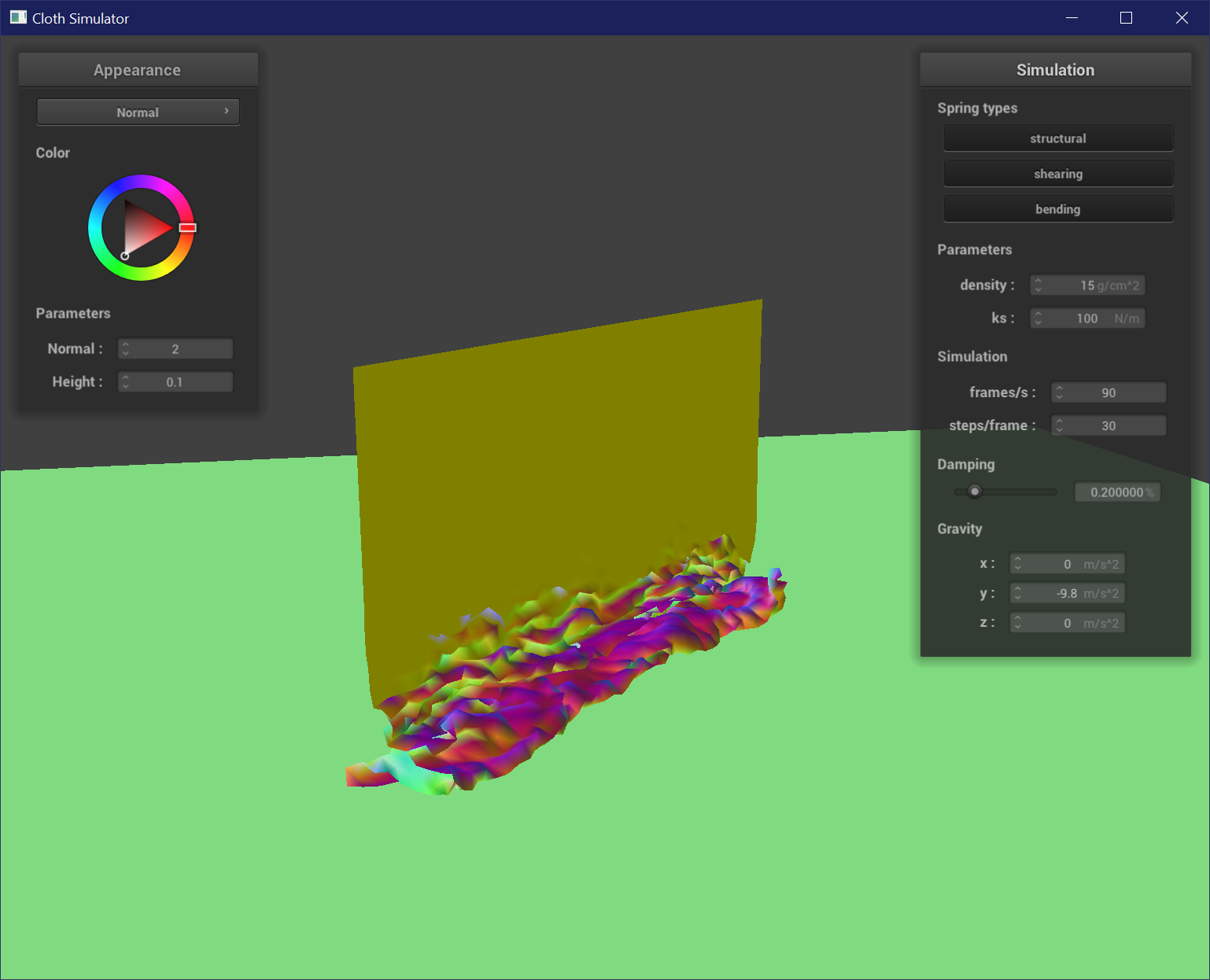
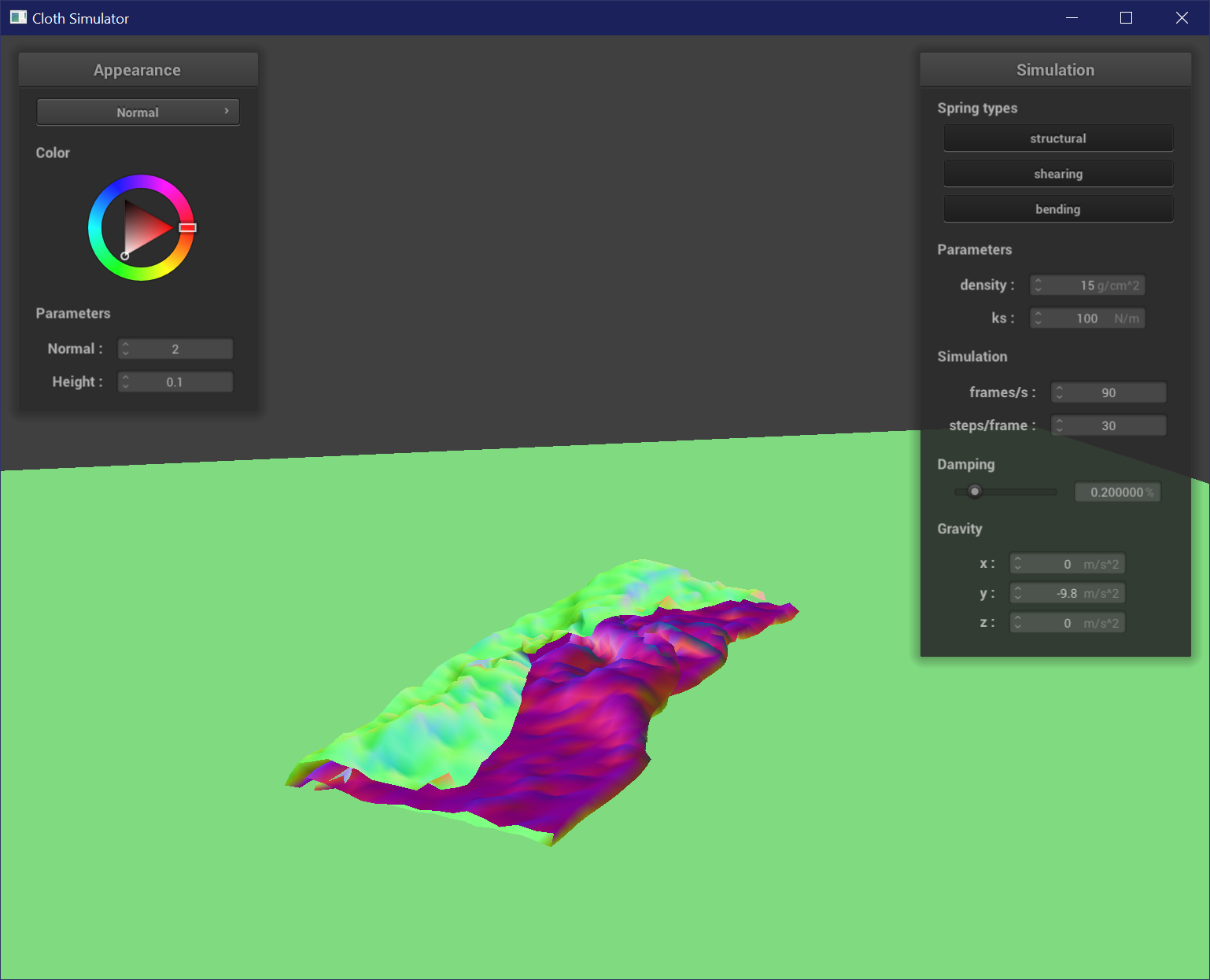
Damping helps simulate energy loss, and so higher damping values result in a faster settle into a resting state. Low damping values result in the cloth acting more jittery, and does not settle to a resting state as quickly, or even at all. It also reacts more violently to any movement among the point masses, and is very wrinkly. High damping values settle to a resting state almost immediately, and the cloth is overall smoother and less jittery. The cloth also exhibits less wrinkles. A low damping value will have a much more jittery cloth that settles down after a longer time than a high damping value cloth.

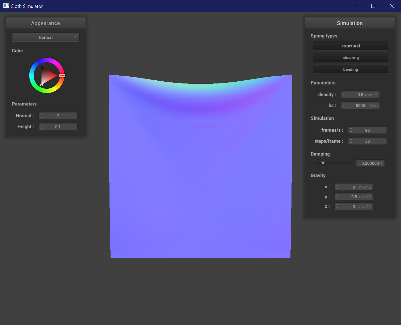
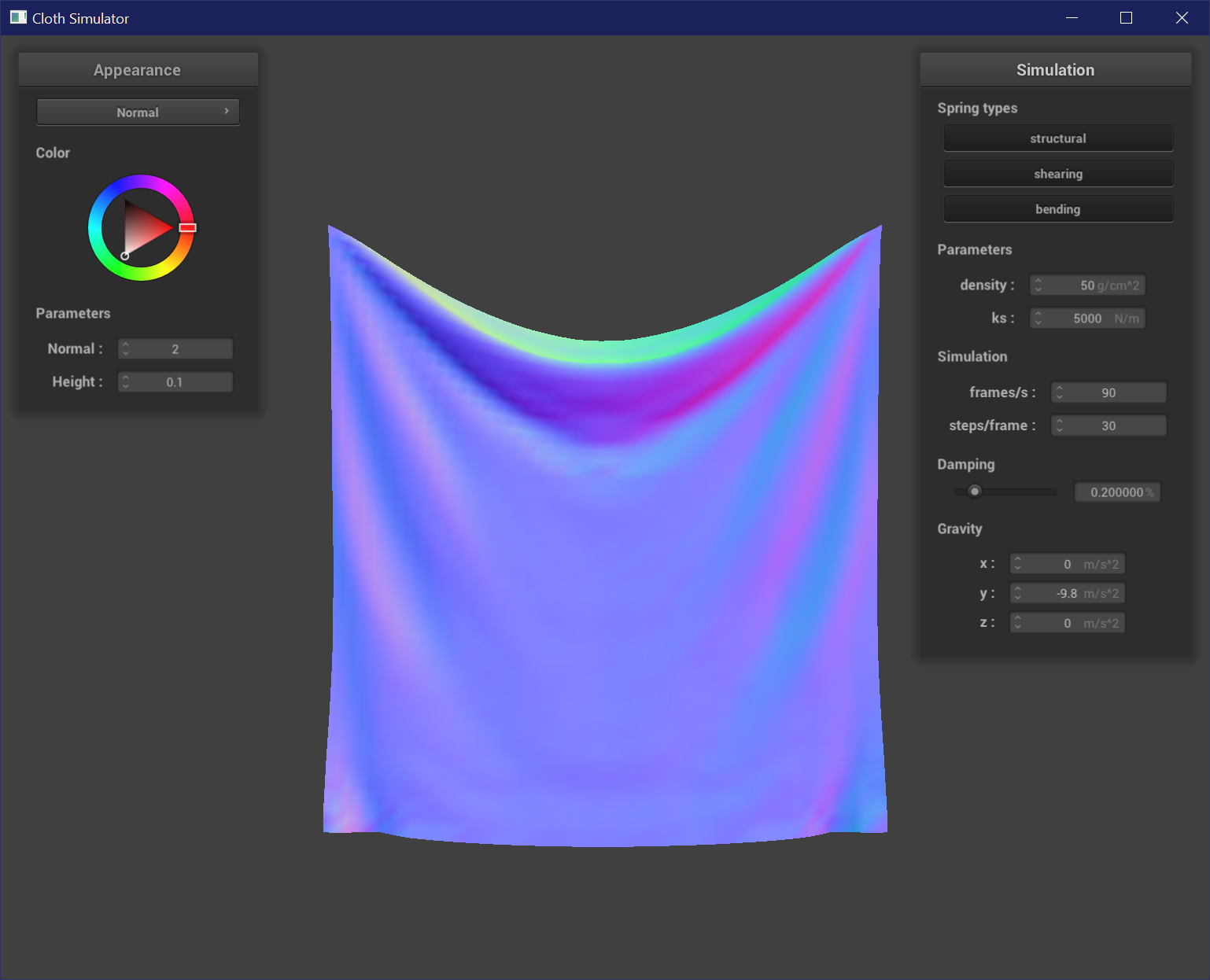
Varying Density

Density affects the mass of the cloth. This affects the "weight" of the cloth, and so with higher densities the cloth appears to hang lower from the pins. The creases are also more prominent in a cloth with high density. A high density cloth will sink lower when the simulation is played than a low density cloth. A low density cloth also maintains its square shape because there is less of a pull on the springs.

Varying Spring Constant

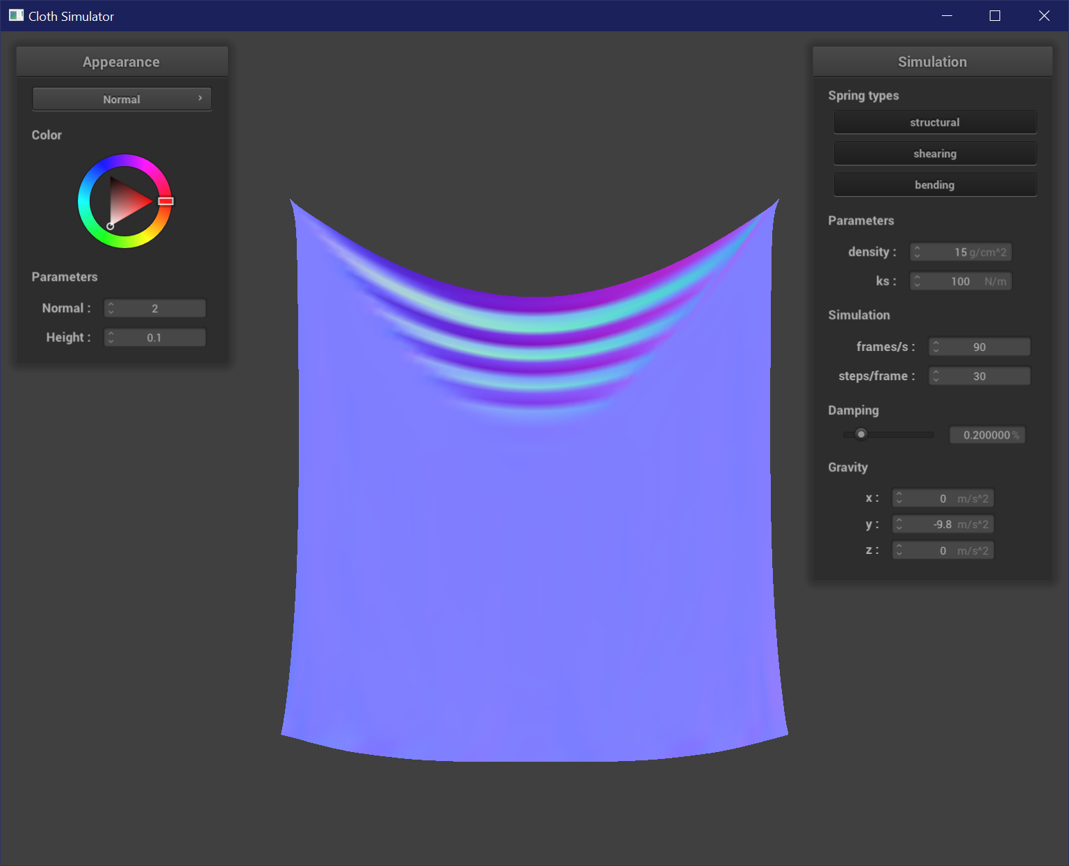
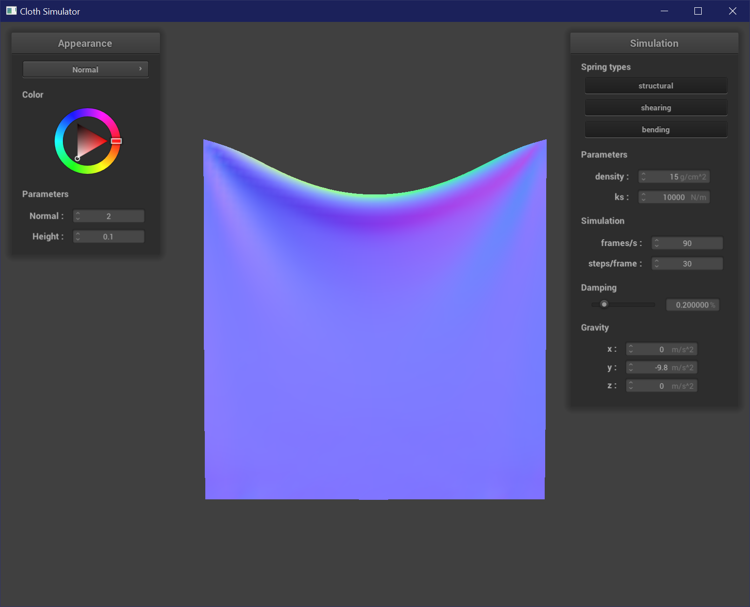
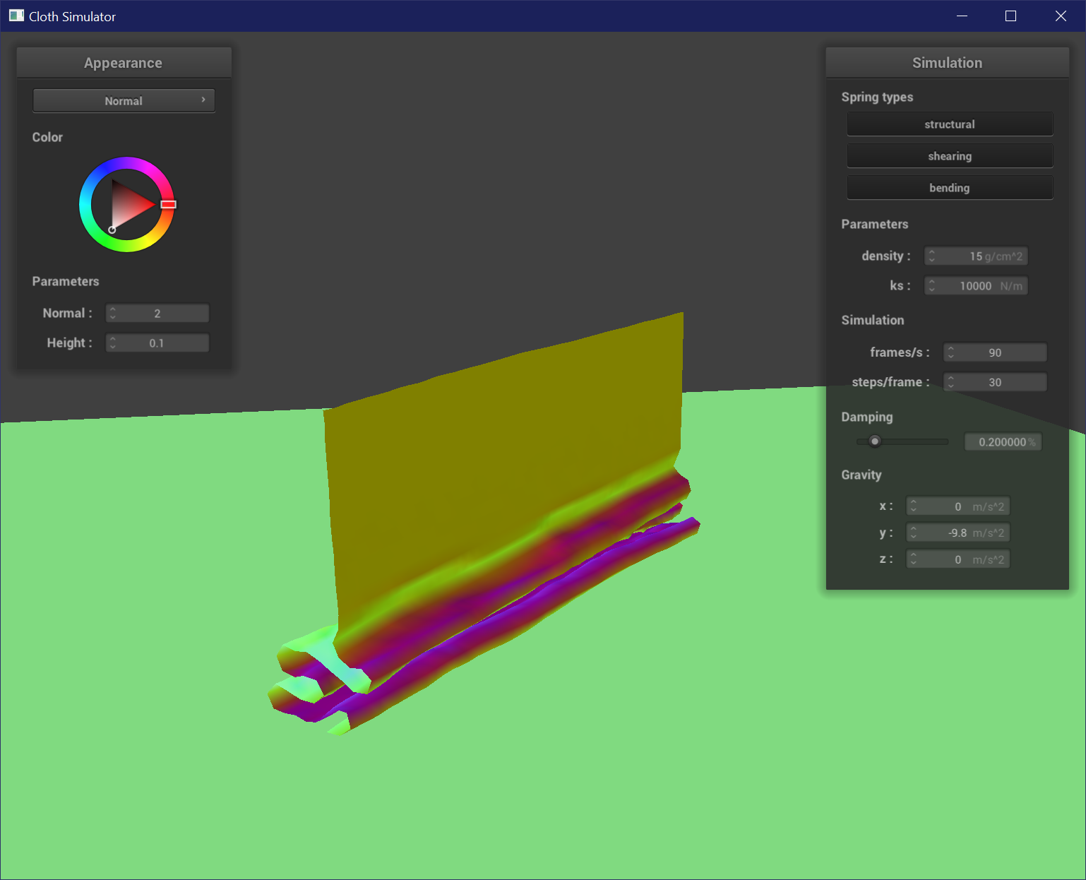
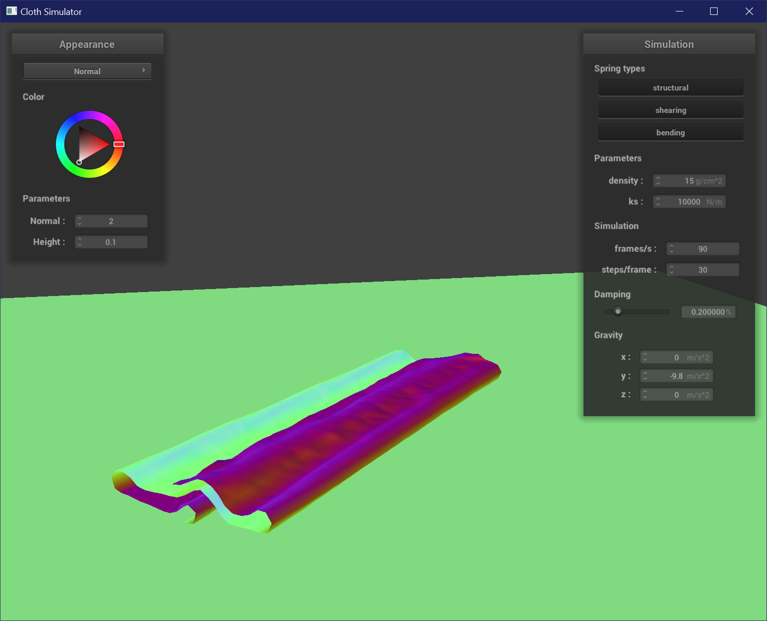
The spring constant affects the strength / stiffness of a spring. A low spring constant results in a more flexible cloth because the springs are weak, which results in the cloth sinking down and forming many tight creases. The edges of the cloth are also pulled down with more gravity. A high spring constant results in a stiffer cloth that does not crease or bend as much.

Part III: Collision with Other Objects

Collisions use similar math to the ray-intersection tests from project 3, in order to find if a point intersects a primitive surface. For a sphere, I first checked if a point is on or inside a sphere, and then created a tangent vector by taking the vector from the point and the origin scaled by the radius and shifted by the origin. I then corrected the position of the point by the tangent to push up a point atop the sphere by its last position + correction * (1 - f).

For a plane, I checked the dot products of the point and plane normals to confirm if a point crossed the plane between its last and current position. I then created a tangent vector by taking position - dot(position - point, normal) - offset * normal. I then corrected the position of the point by the tangent to push up a point above the plane by its last position + correction * (1 - f).

Varying Spring Constant

The spring constant affects the strength / stiffness of a spring. As spring constant increases, the cloth is stiffer and drapes less over the sphere, resulting in the cloth wrapping around less of the sphere and forming less and wider creases.

Part IV: Self-Collision

To implement self-collision, I used spatial hashing to partition the 3D space of points into several bins based on the nearest box with dimensions w * h * t where w = 3 * width / num_width_points and h = 3 * height / num_height_points and t = max(w, h). The point is then hashed using its truncated value and a quadratic function of x * 31^2 + y * 31 + z. I then built a map of these hash values as keys and a vector of points that hash to these keys. For each point in a bin, if any points are within 2 * thickness distance of each other, I created a correction vector that would adjust the position of the current point so it would be placed at the average of all the correction distances scaled by simulation_steps. This position correction then allows the cloth to appear to be self-colliding by prevent points from intersecting or clipping with each other.

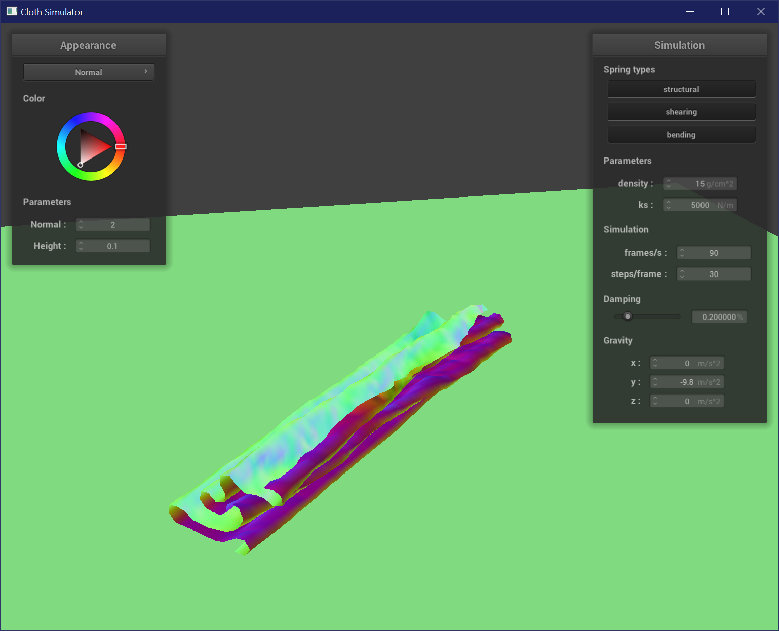
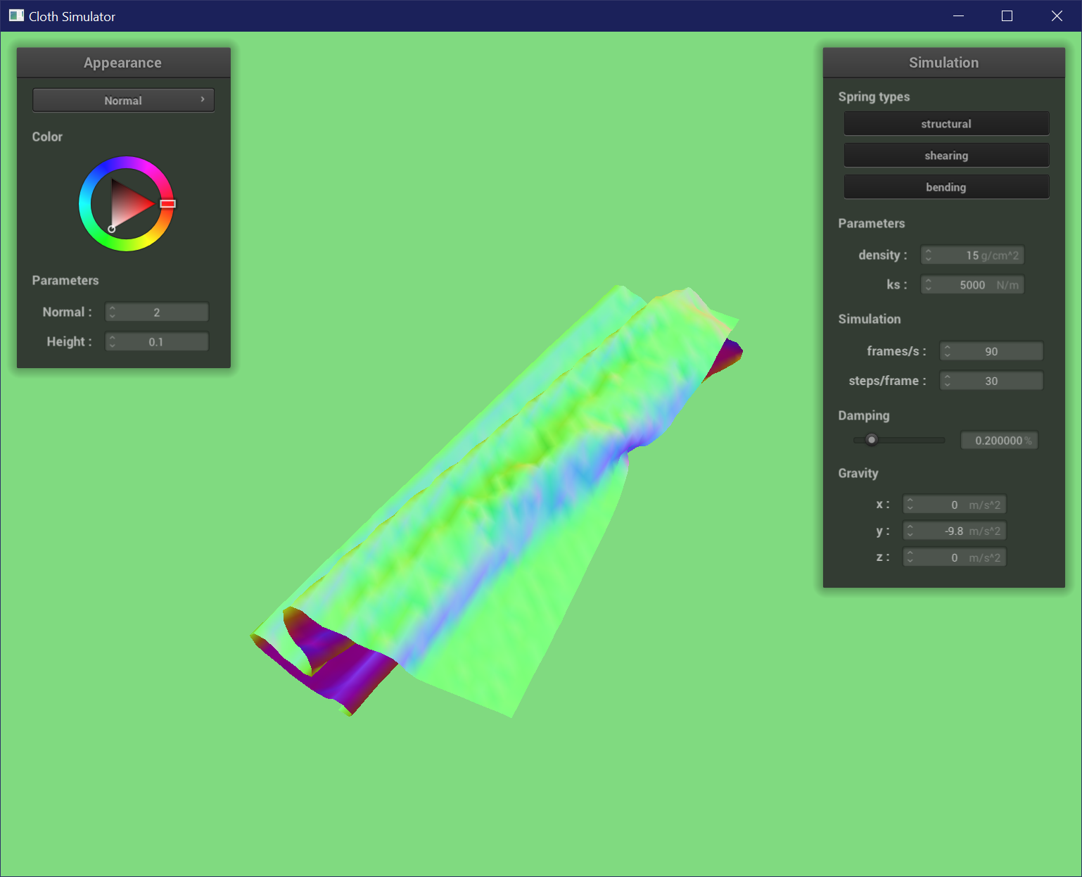
This shows the cloth at 3 stages of its fall. Notice how instead of clipping into itself, it folds over itself and settles into a folded and creased pile.

Varying Density

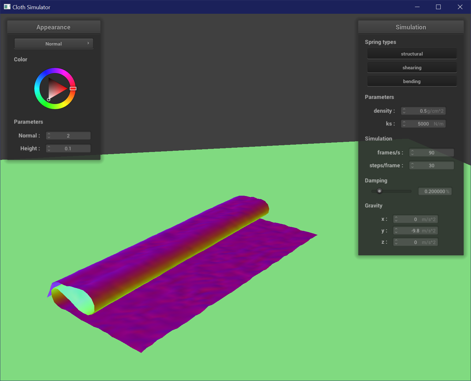
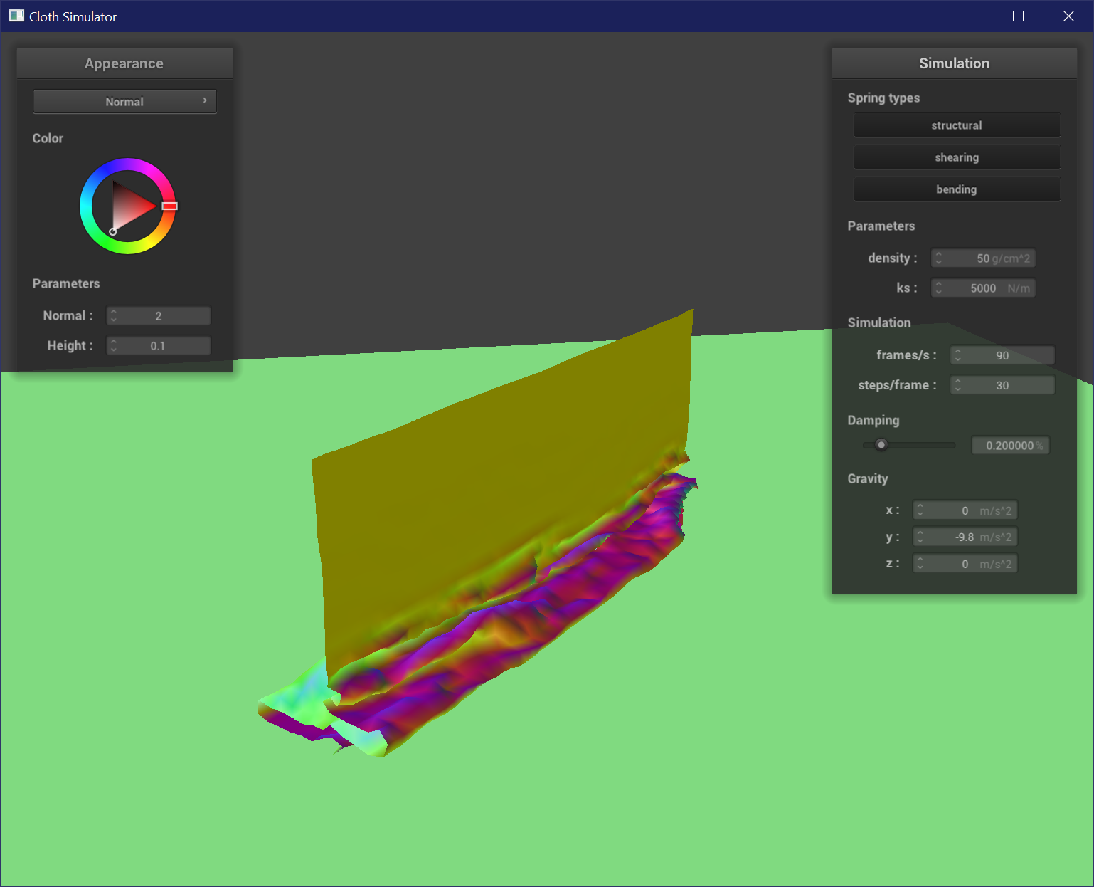
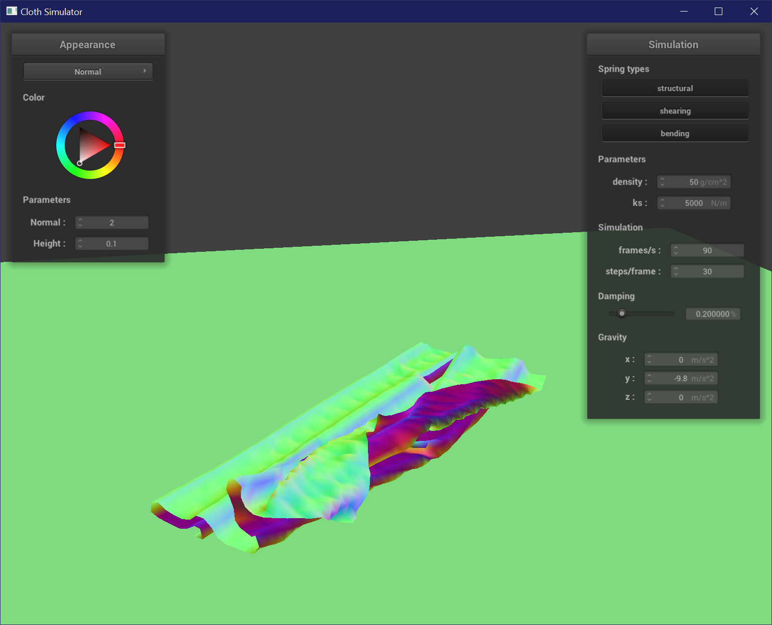
A low density cloth falls very smoothly and forms large parallel folds. The self-collision propagates a wavelike ripple up the cloth. A high density cloth has many more small wrinkles and creases and forms small, uneven folds. It does not fold over as cleanly as a low density cloth.

Varying Spring Constant

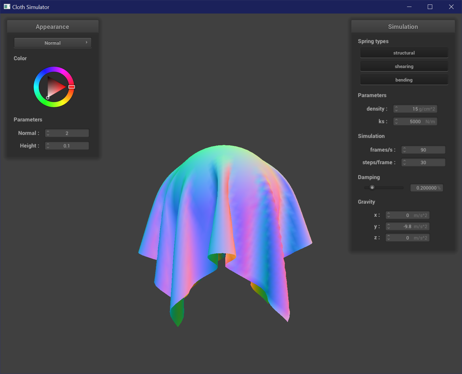
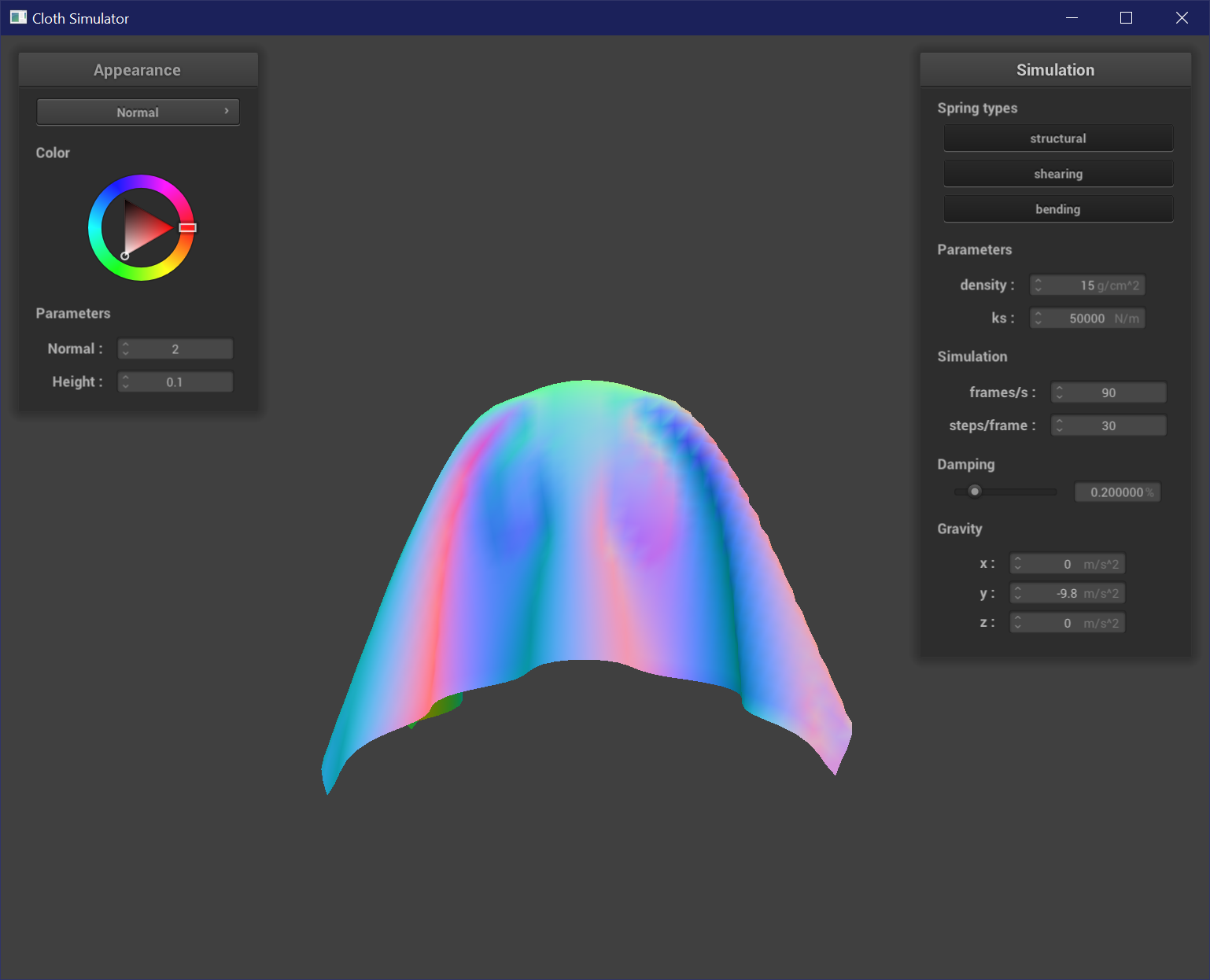
A low spring constant results in a wrinkly cloth that is very jittery as it self-collides at a smaller scale from looser springs. A high spring constant results in very smooth and even folds, and tends to lay flat once it is at rest. The cloth is not as jittery because the springs are stiffer.

Part V: Shaders

A shader program written in a language like GLSL defines how the surface attributes and normals are affected to mimic real life material properties such as reflections, refractions, and matte surfaces. It takes in inputs such as positions and returns outputs that are represented by the renderer. Shader programs can also run in parallel on GPU instead of CPU, leading to several speedups.

A vertex shader applies transformations to each vertex on a mesh, which is useful especially in the case of displacement mapping, where the positions and normals of each vertex are shifted according to a texture map. On the other hand, a fragment shader in GLSL writes out the actual colors and attributes associated with each fragment, per-pixel, including effects like reflections and transparency. Transformations applied in the vertex shader are inputted into the fragment shader to output the final color of the pixel.

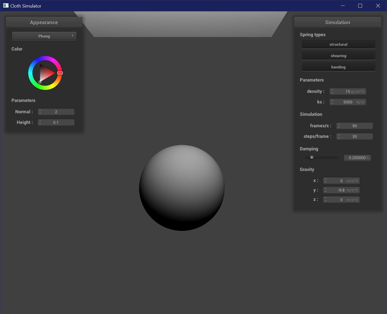
Blinn-Phong Shader

The Blinn-Phong shader model is comprised of 3 main components: the ambient component, the diffuse component, and the specular component, which together creates a shader that has a diffuse color and some reflective or specular properties. The Blinn-Phong shader equation is: L = k_a * I_a + k_d * (I / r^2) * max(0, dot(n, l)) + k_s * (I / r^2) * max(0, dot(n, h))^p. K_a, k_d, and k_s are the ambient, diffuse, and specular constants, respectively. This formula can be broken up into the following to represent the individual components:

• Ambient: k_a * I_a
• Diffuse: k_d * (I / r^2) * max(0, dot(n, l))
• Specular: k_s * (I / r^2) * max(0, dot(n, h))^p

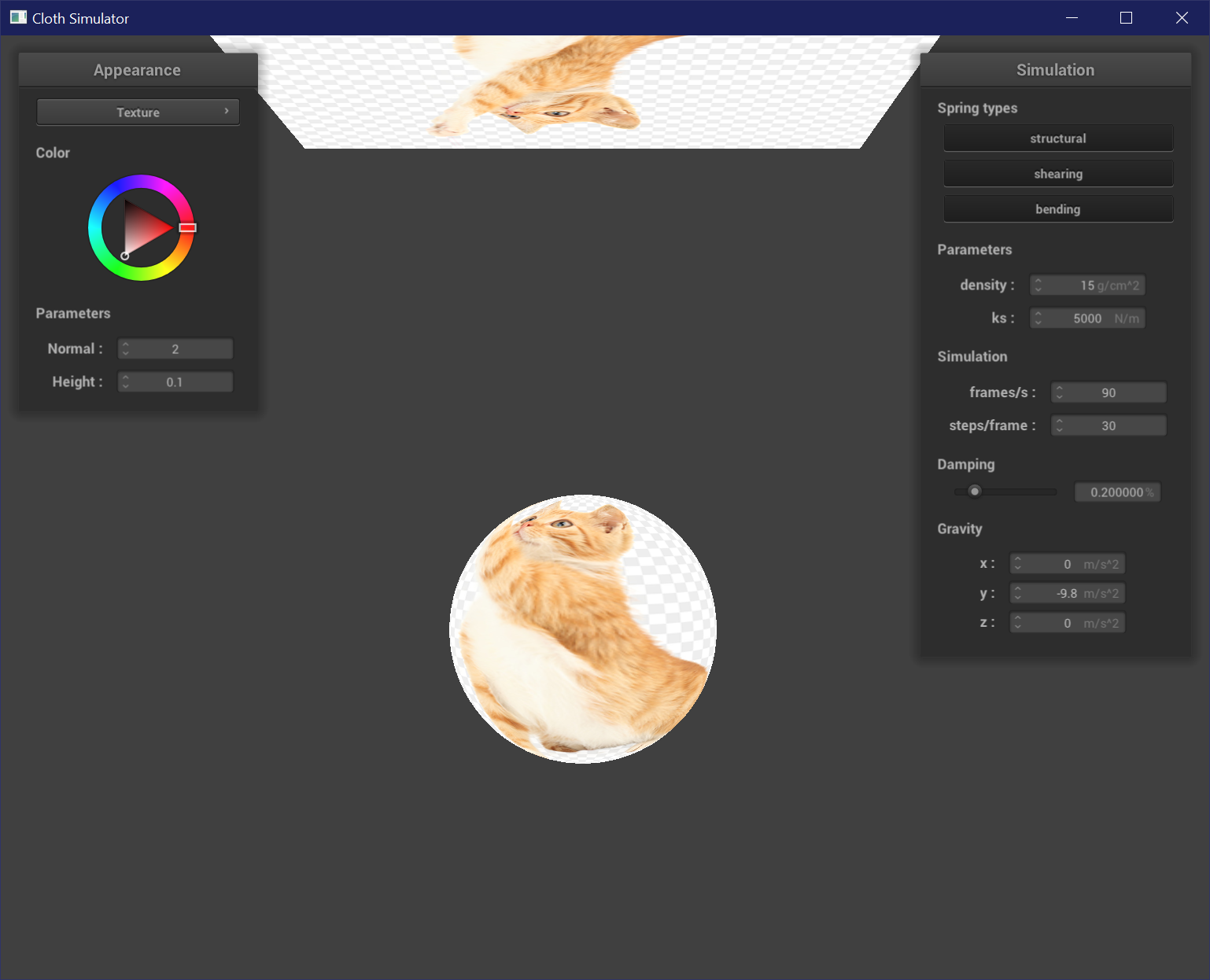
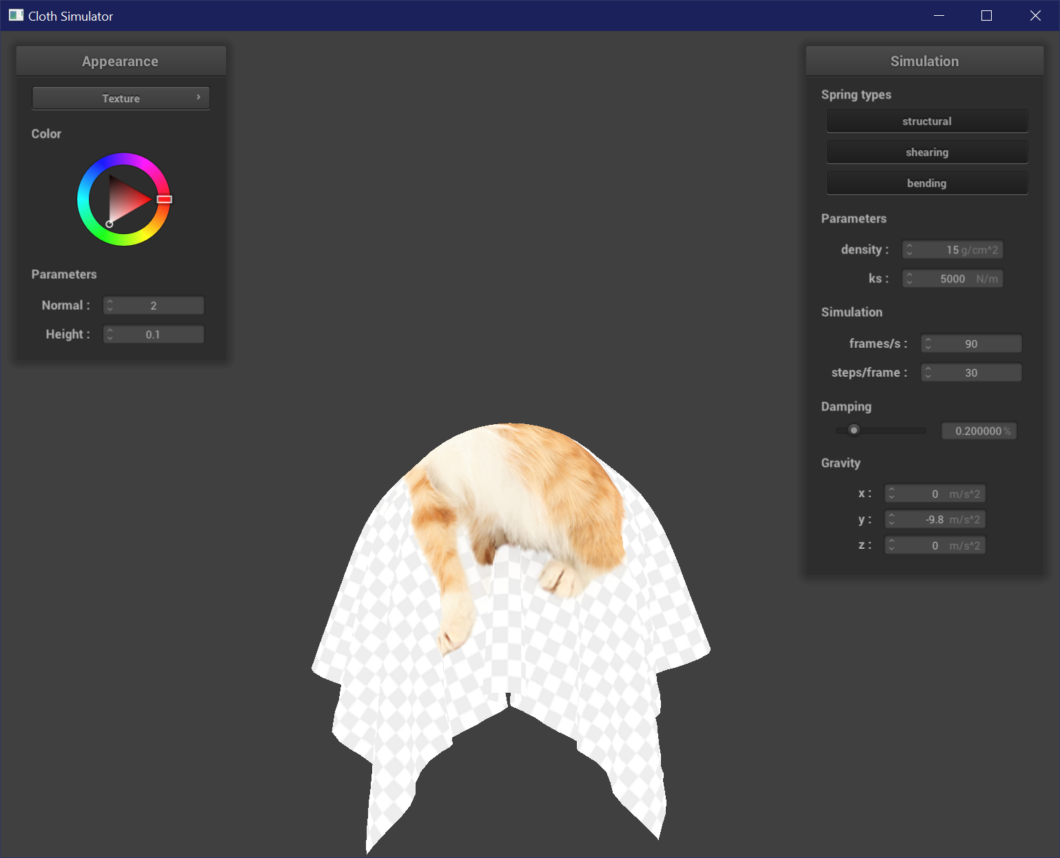
Texture Shader

Here I applied a custom texture and inputted it into a texture sampler in the fragment shader.

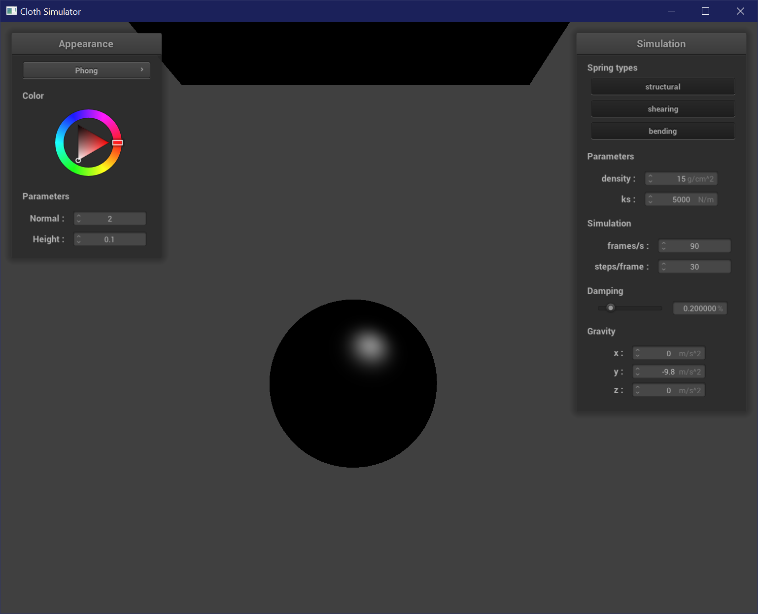
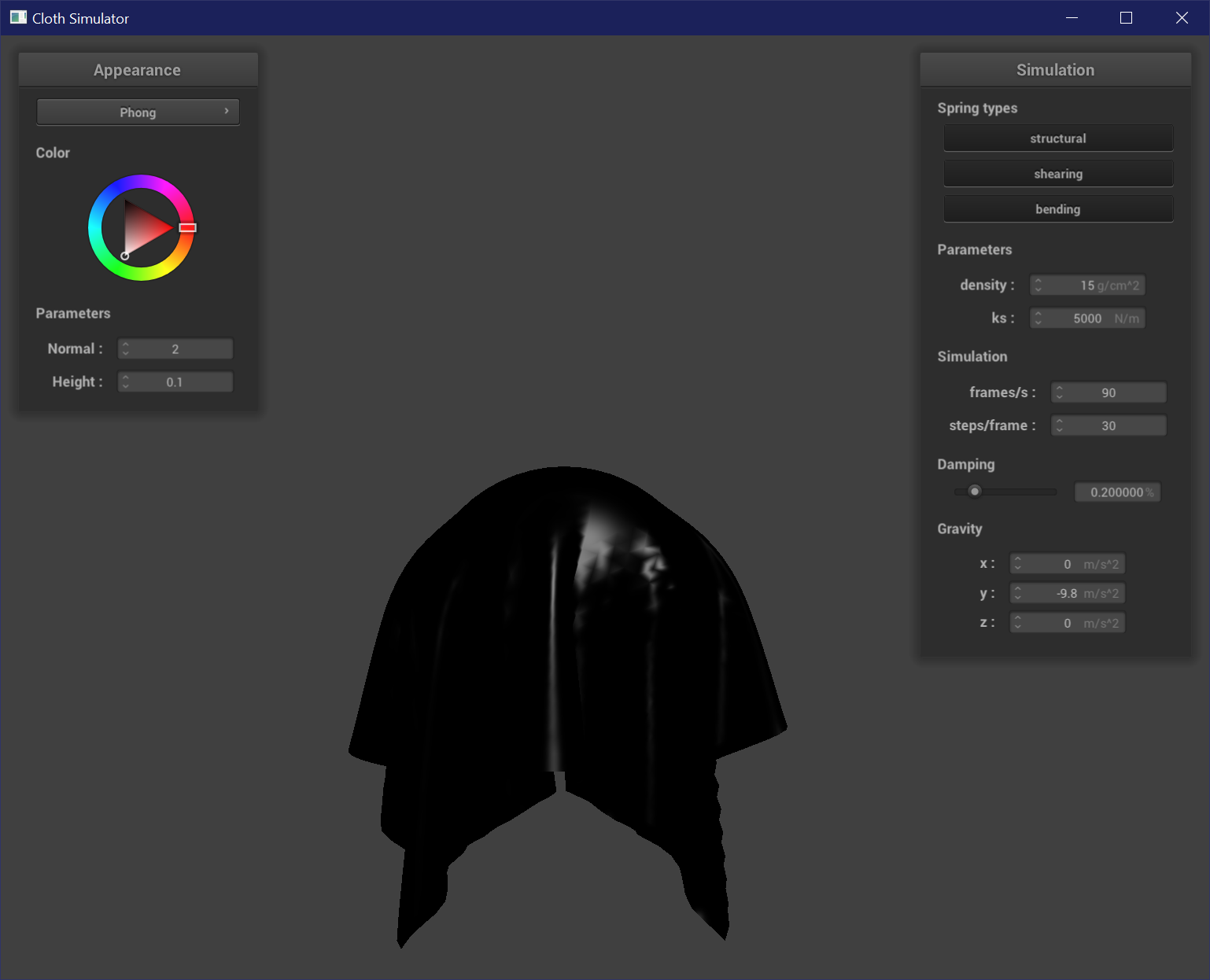
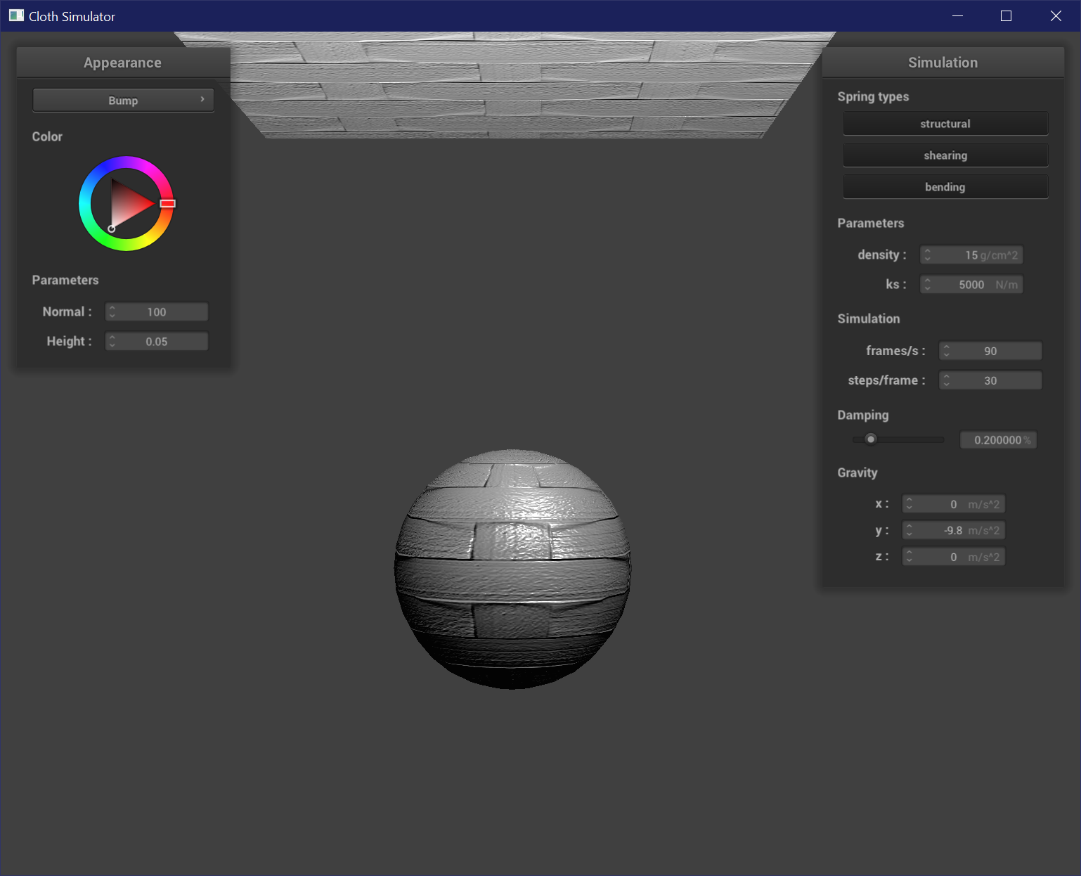
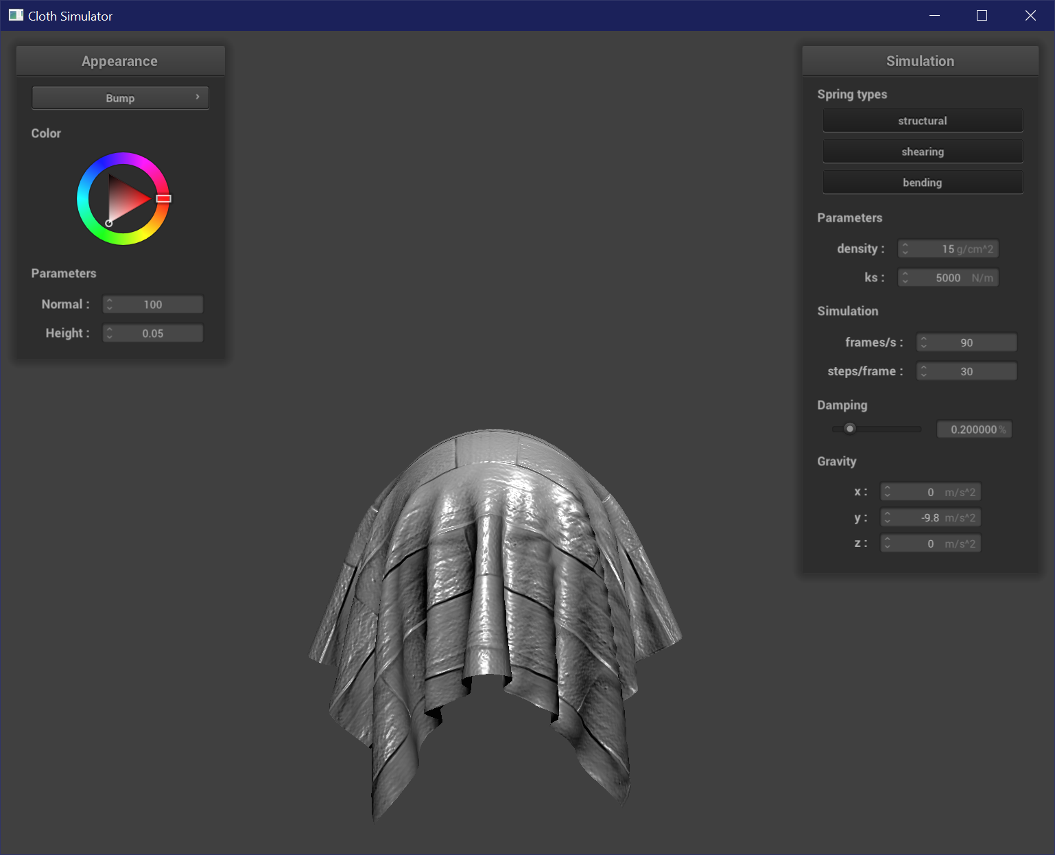
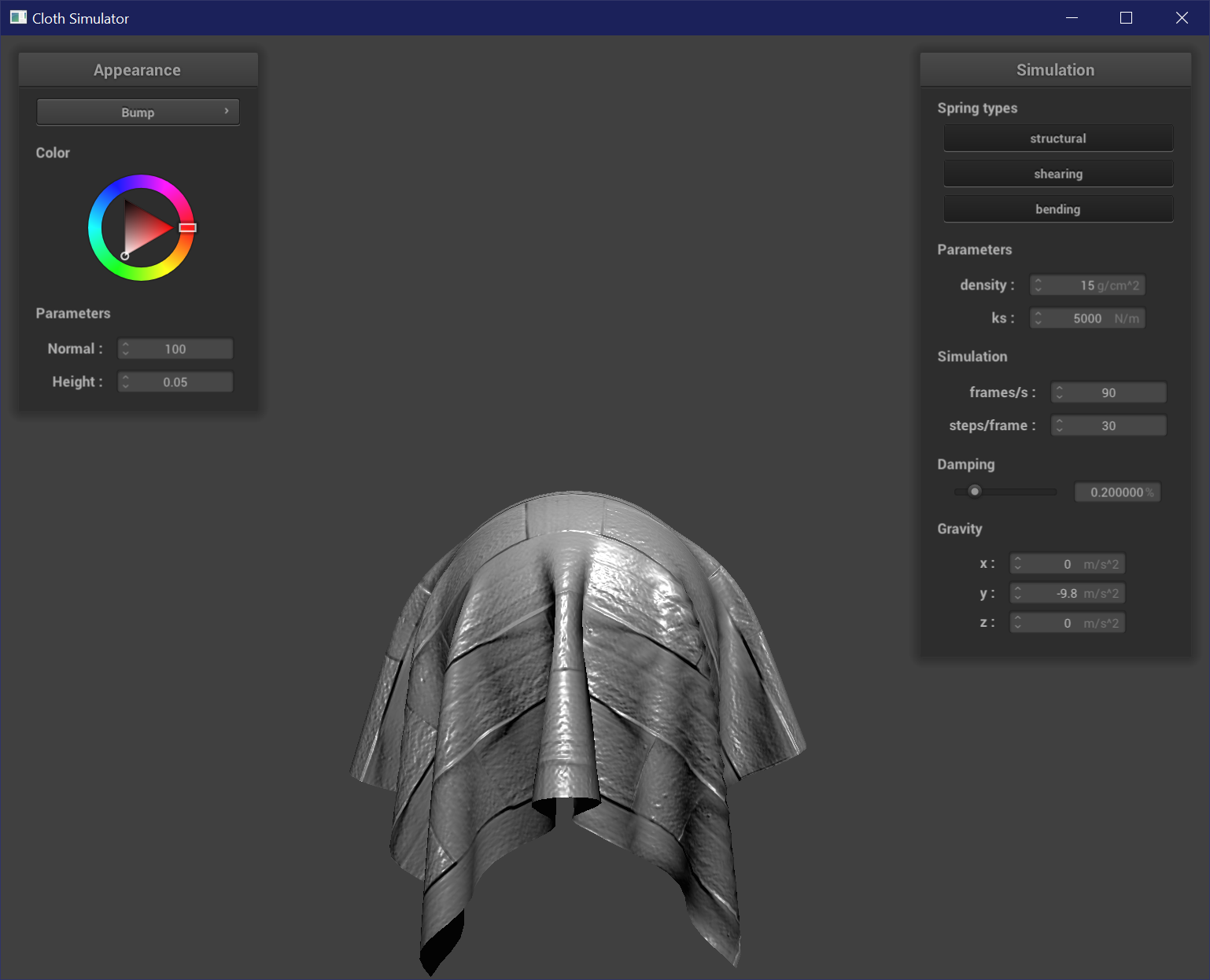
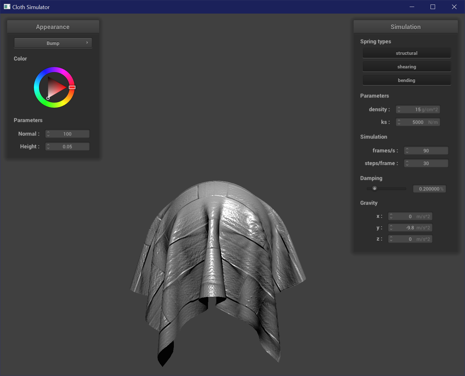
Bump Mapping

Bump mapping is a fragment shader code which modifies the normals of each fragment to mimic specular and shadow details such as peaks and grooves, without changing the actual geometry of the mesh. Most of the values are in model space, but we can calculate the changes in normals in object space and then transform it back to model space with the tangent-bitangent-normal (TBN) matrix, which consists of the tangent vector, the normal vector, and the bitangent (the orthogonal cross-product of the tangent and normal). To compute the new normals, we use a height map sampled at texture coordinates u and v. The changes in our heights are represented by dU = (h(u + 1 / w, v) - h(u, v)) * k_h * k_n and dV = (h(u, v + 1 / h) - h(u, v)) * k_h * k_n. k_h and k_n are the height and normal scaling factors. The new local space normal is n_o = (-dU, -dV, 1). It is then transformed back into model space with n_d = TBN * n_o.

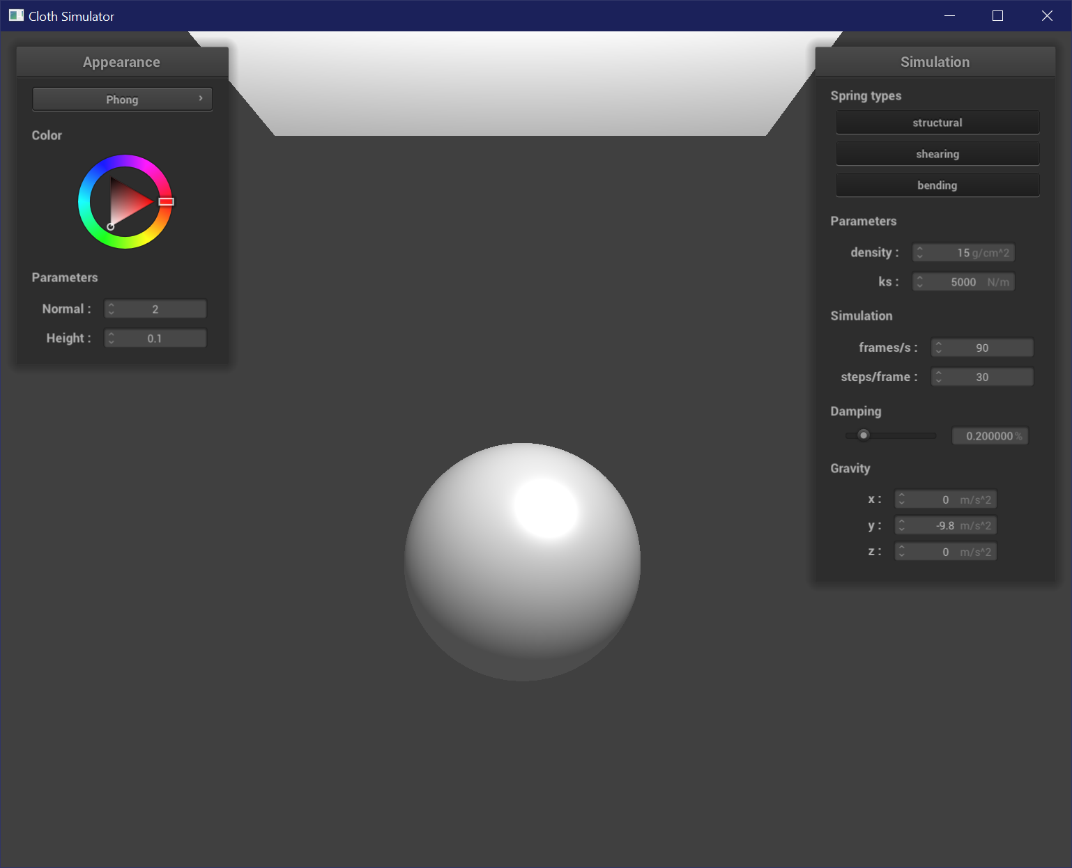
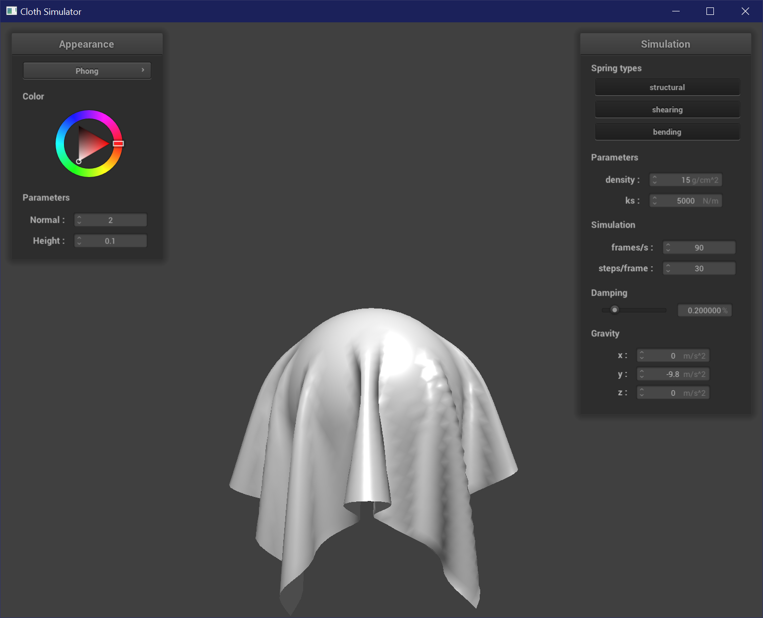
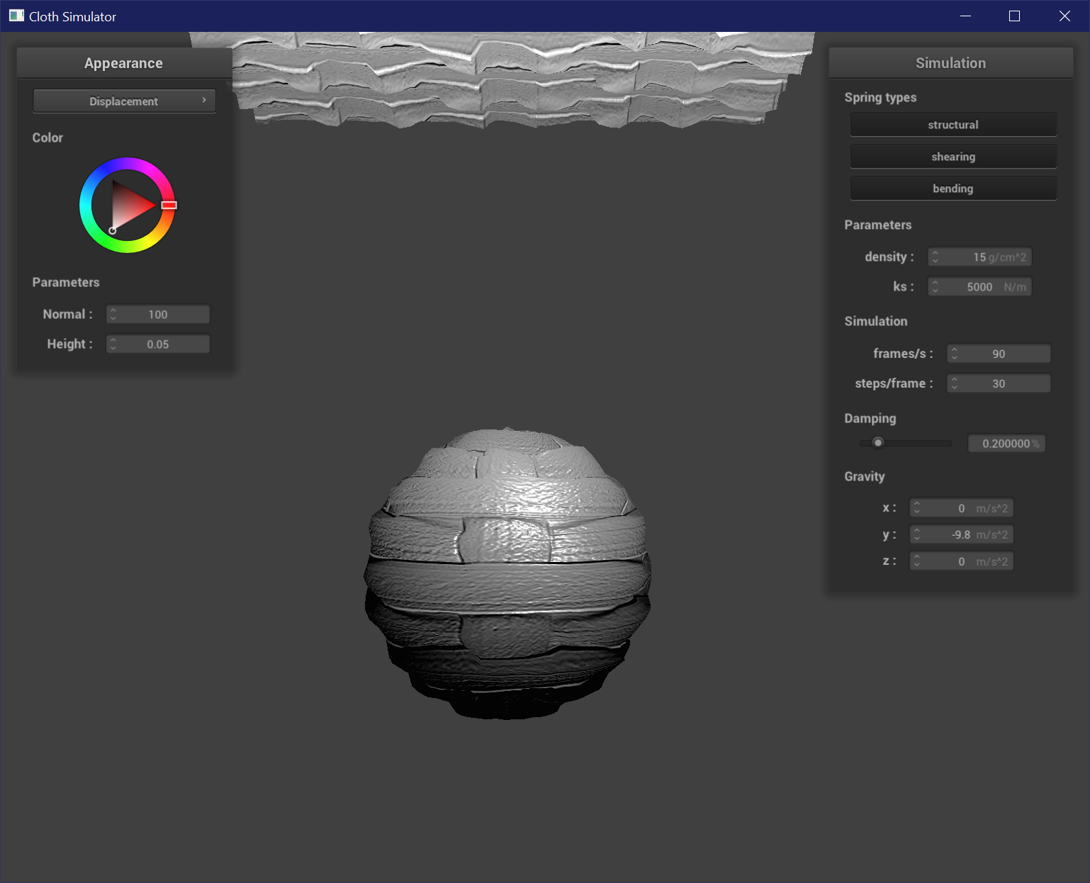
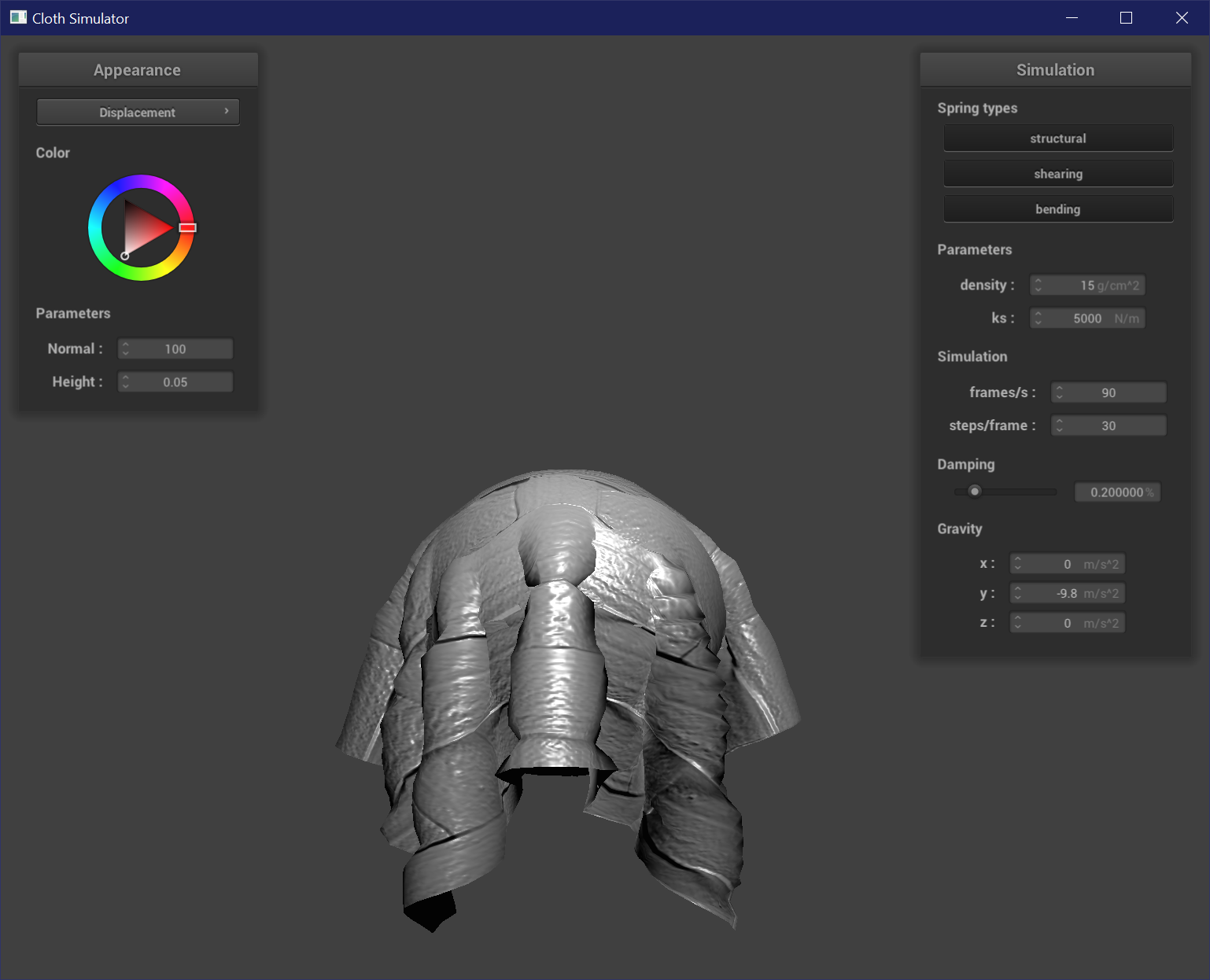
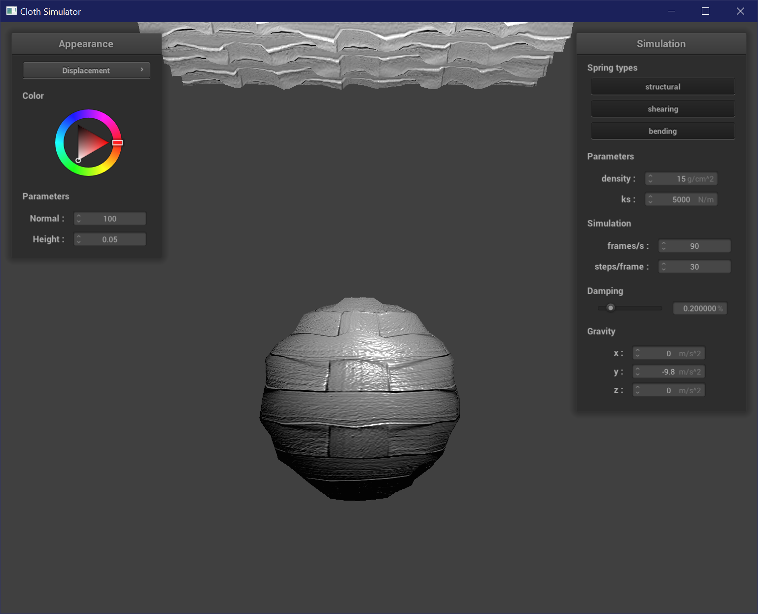
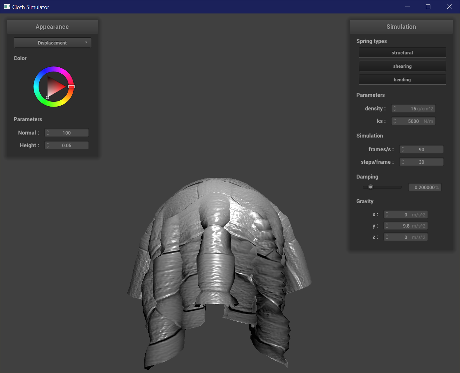
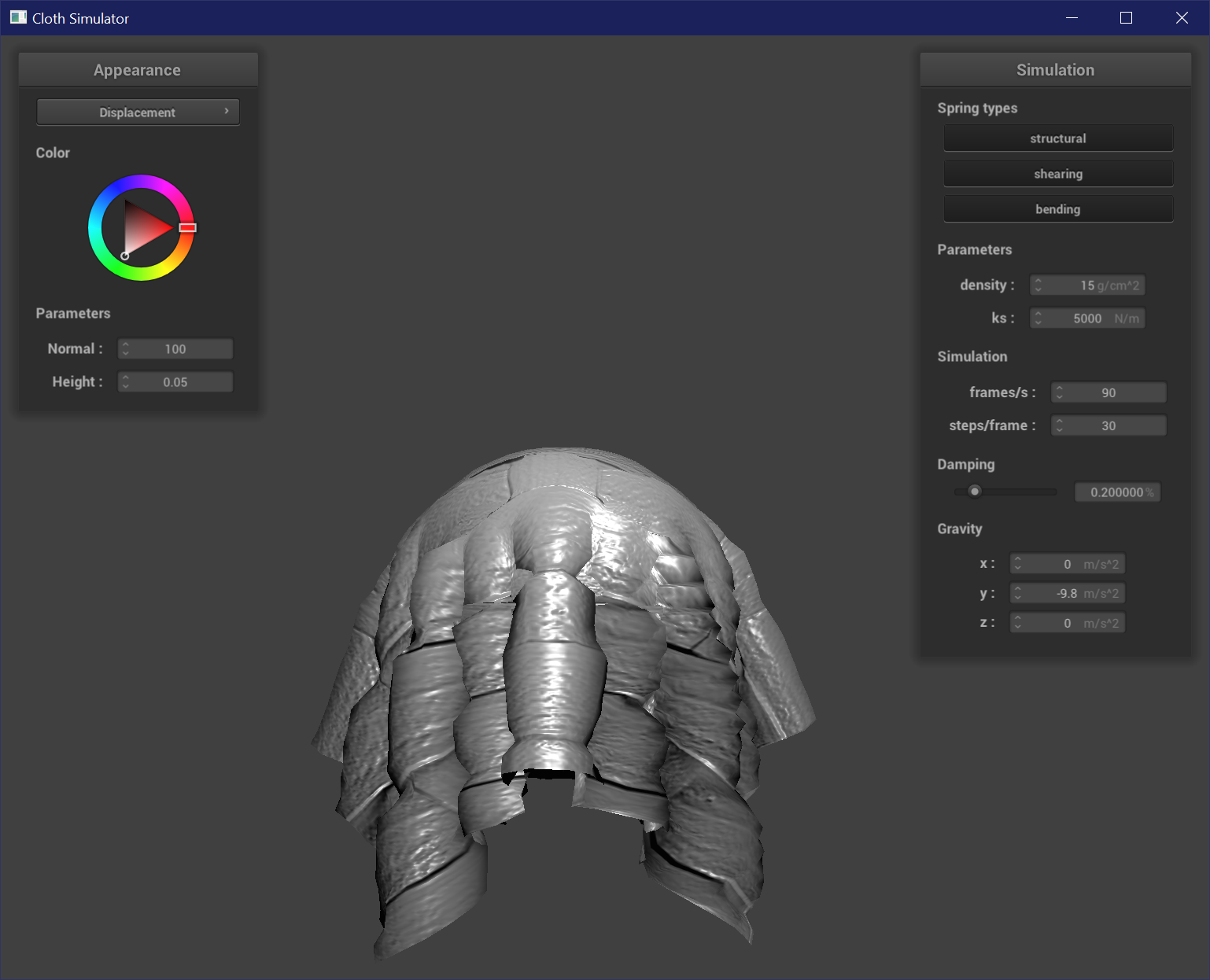
Displacement Mapping

Displacement mapping is like the physical manifestation of bump mapping. It uses the same calculations in the fragment shader to shift normals and represent the reflections and shadows of grooves, but in addition changes the actual mesh geometry of the vertices as well. To change the vertex positions, the vertex shader also samples from the height map and changes the position of each vertex by position + normal * h(uv) * height_scaling_factor. Now the grooved and raised parts of the texture are actually grooved and raised.

Resolution

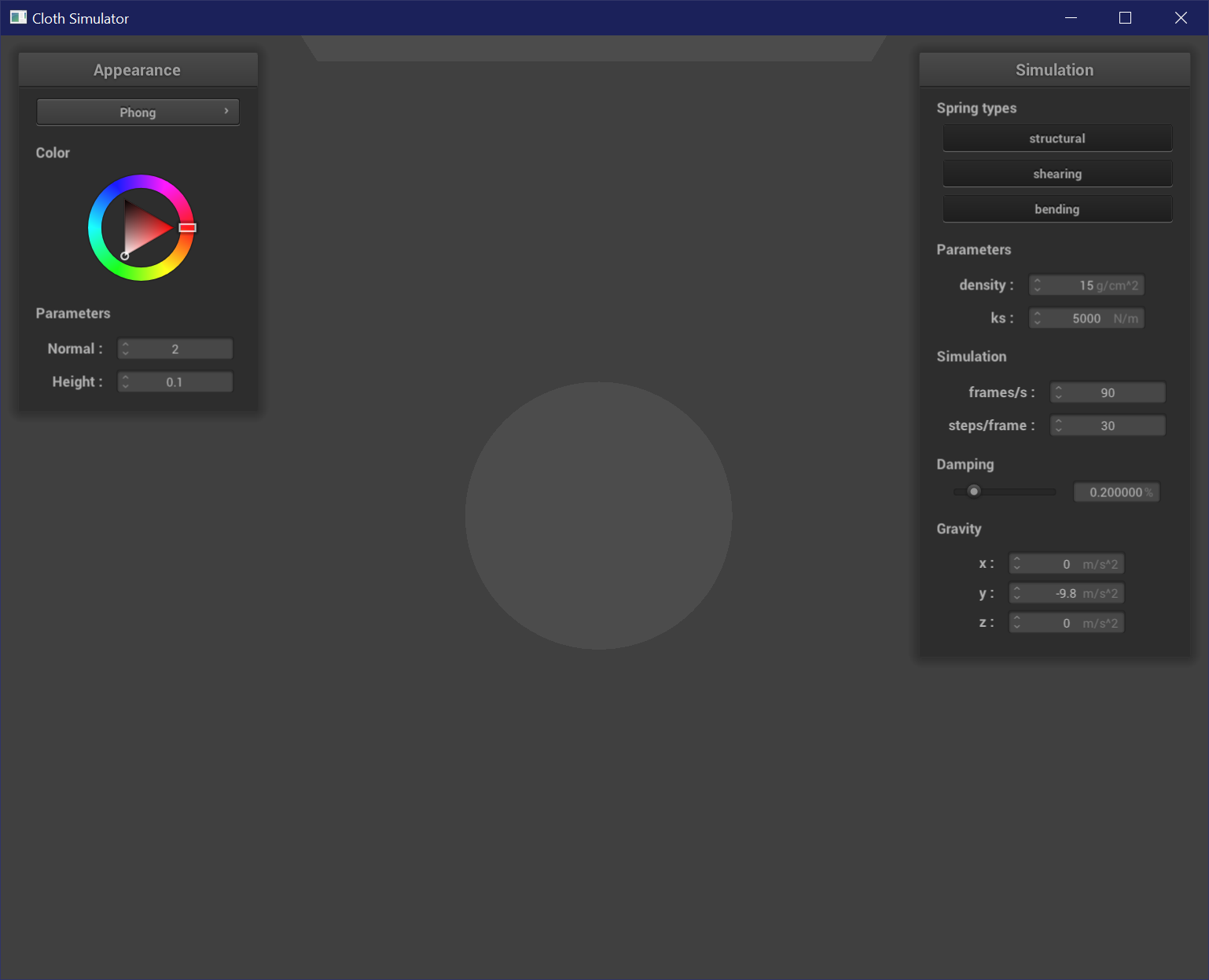
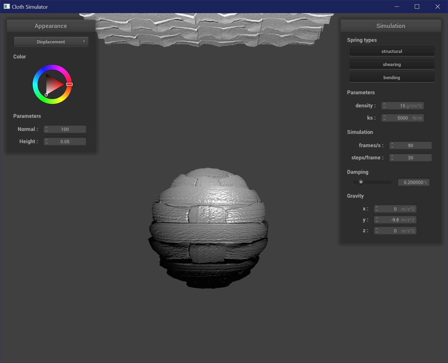
The resolution of the sphere mesh does not show any clear difference when used for bump mapping.

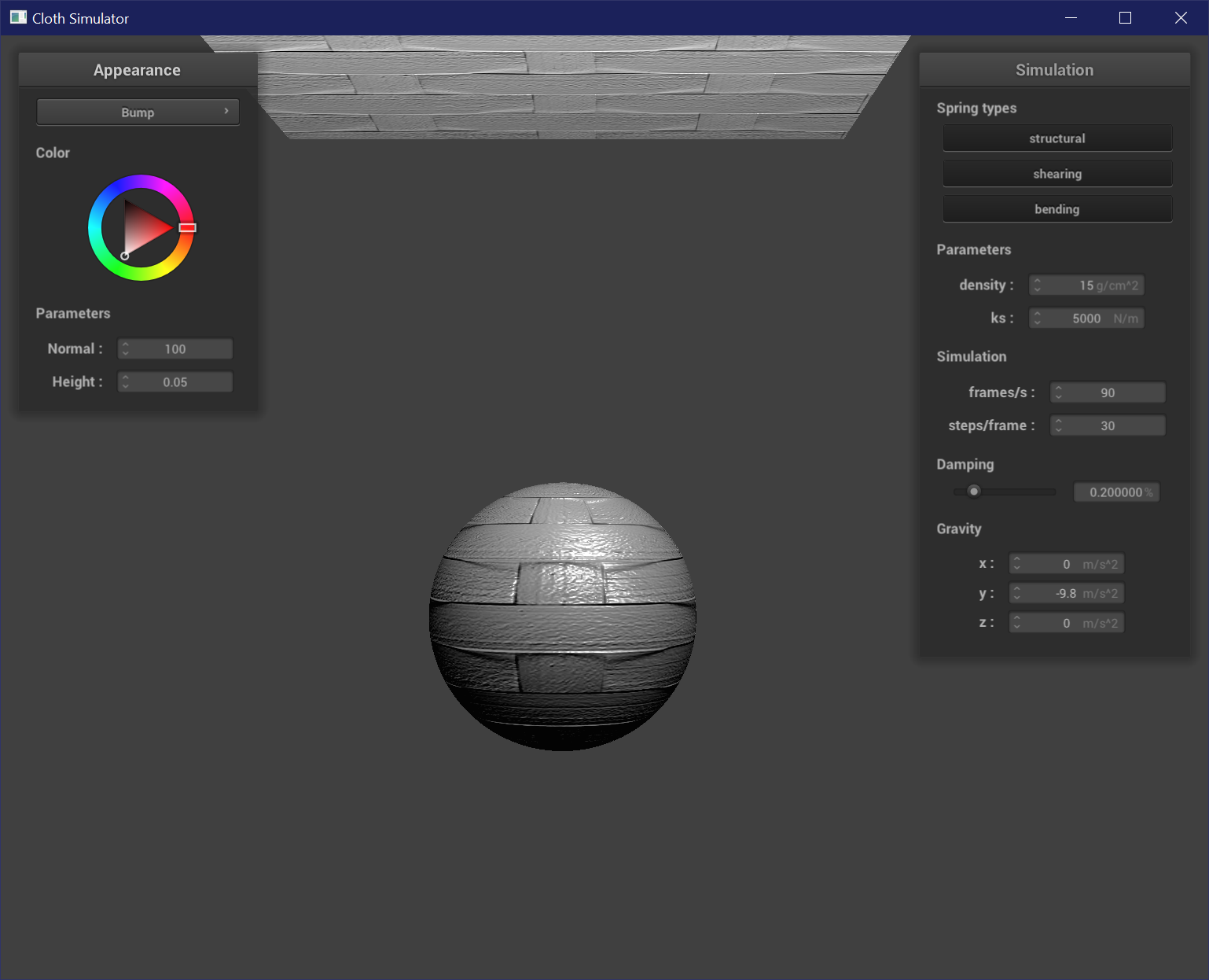
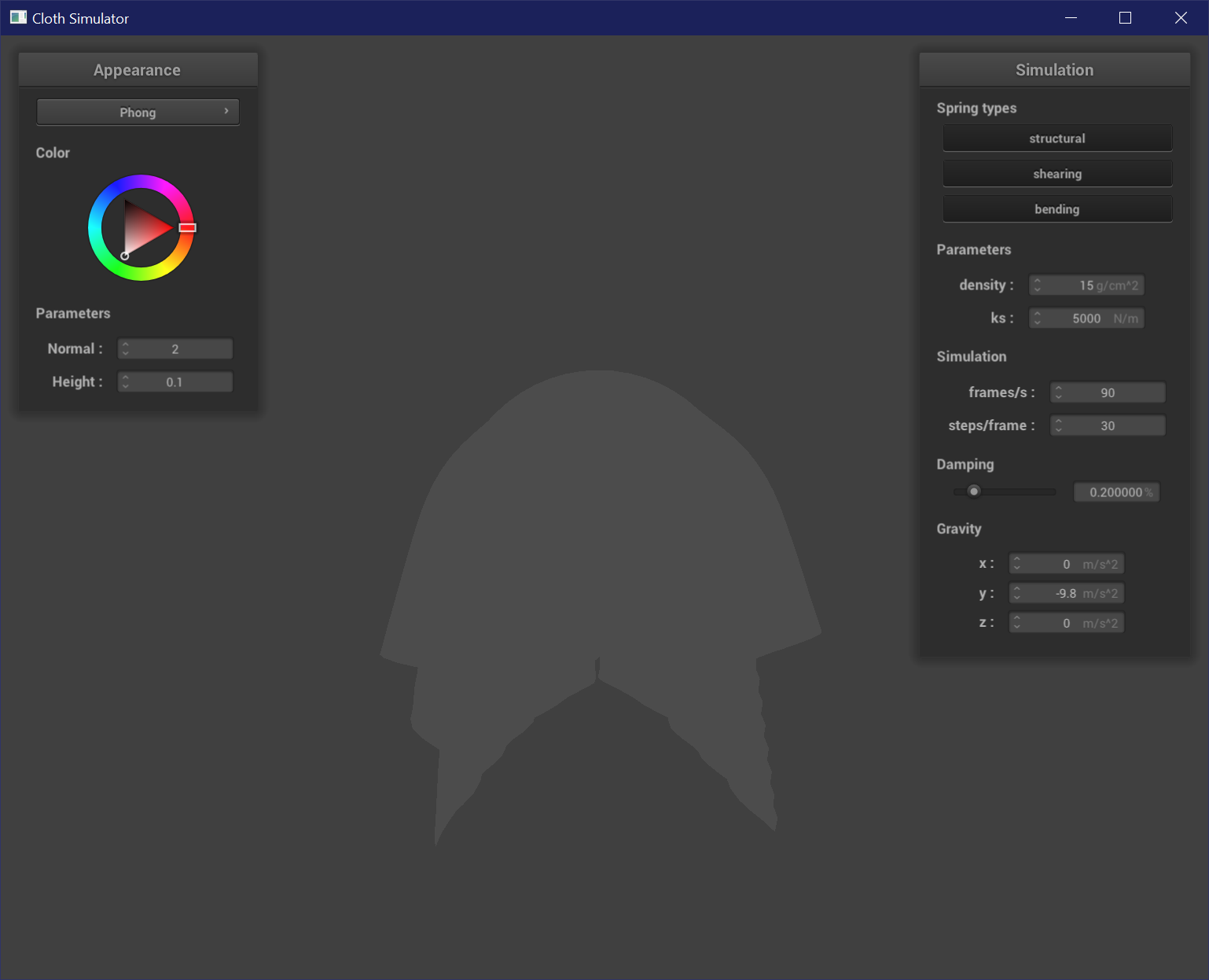
The resolution of the mesh is more evident when used for displacement mapping. At higher resolutions, the displacement effect follows the texture map more closely because there are more vertices to sample from the texture map. The sphere is less sharply affected by low and high points, and has a less prominent stair-like or fresnel-like pattern on its surface at higher resolutions. This is more clearly seen at the pole of the sphere, where at resolution = 16 the top has a peak.

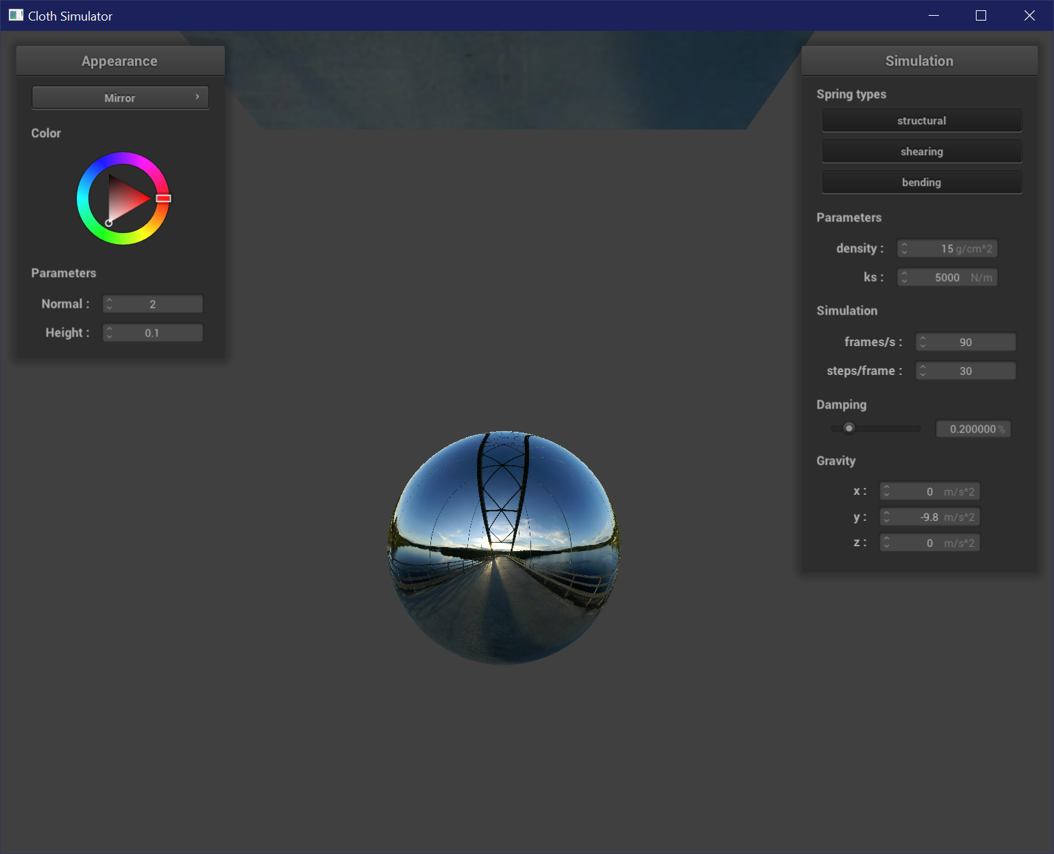
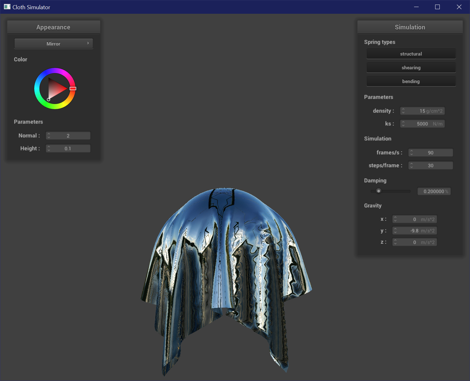
Mirror Shader

To create a mirror shader, the fragment shader just needs to use the reflection equation to reflect incoming and outgoing rays along the normals of the mesh. It is reflecting a cubemap environment texture map.