Pathtracer I
Implemented a basic ray tracer for diffuse BSDFs, optimized with basic speed ups such as bounding volume hierarchies. The ray tracer supports direct and indirect illumination by tracing rays through bounces in the scene using both uniform hemispherical lighting and importance sampling of lights. Adaptive sampling helps reduce overall noise in the final renders.
Section I: Ray Intersections
Part 1: Ray Generation and Scene Intersection
Task 1: Generating Pixel Samples, Task 2: Generating Camera Rays
First, to generate rays in the camera space I first generated ns_aa rays by each sampling from a uniform unit square and generating camera rays in image space with offsets of (sample_x + x) and (sample_y + y), normalized by the width and height of the image. I then updated the pixel's spectrum with the estimated radiance normalized by number of samples. Generating the ray itself involves converting from image space to camera space by converting the (0, 0) equivalent in image space to (-tan(0.5 * hFov), -tan(0.5 * vFov), -1), and (1, 1) to (tan(0.5 * hFov), tan(0.5 * vFov), -1). I then converted the vector that converts the ray's x and y coordinates to world coordinates, and generated a ray with this new offset and set the ray's min and max to nClip and fClip respectively.
Task 3: Ray-Triangle Intersection, Task 4: Ray-Sphere Intersection
To implement triangle intersection, I used the Moller-Trumbore algorithm. Moller-Trombore requires using a ray's
origin and direction, as well as a triangle's 3 points in space, to calculate barycentric coordinates to get an
intersection point on the triangle plane. If the point is within the triangle (barycentric coordinates are positive and
withing (0, 1)) the ray intersects the triangle.
To determine if a ray intersects a triangle primitive, I checked that each of the resulting barycentric
values that result from the algorithm are within (0, 1.0),
intersection time t is greater than 0, and that t is within the ray's min and max t. If all of the above
are satisfied, I reduced that ray's max t value to optimize future intersections, and updated the isect struct with
appropriate values.
To implement sphere intersection, I used the ray-sphere intersection algorithm that requires solving for for the intersection
of (ray_origin + t * ray_direction - sphere_origin)^2 - radius^2 to get two t values for each point that
a ray enters and exits a sphere. if these two t values are within the ray's min and max t, then I reduced that ray's
max t value to optimize future intersections, and updated the isect struct with appropriate values.
I render an image to the screen by tracing rays from image space to the camera space and checking if a primitive is intersected; else, draw black.
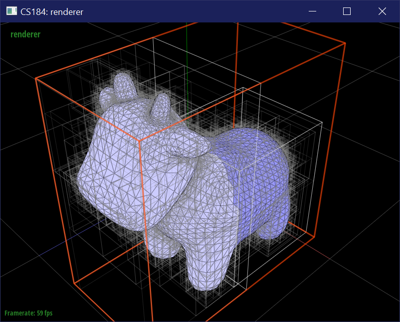
Part 2: Bounding Volume Hierarchy
Task 1: Constructing the BVH
I constructed a BVH to speed up rendering times by not bothering to check primitive intersections if the primitive's bounding box is entirely missed by a ray. To construct the BVH, I first generated the root bounding box by generating the box surrounding the entire mesh by expanding the bounding box starting from individual primitive boxes. Then, I checked if the current node is a leaf. If so, then I populated the node's values appropriately and null'd out its pointers to a left and right child. If not, then I created two vectors to hold the primitives that would go into the left and right child nodes. For each primitive, if its centroid is less than the average centroid of all bounding boxes along the longest axis (my heuristic), I placed it into the left child node. Otherwise, I placed it into the right child node. I then recursively called the bounding box construction algorithm for the left and right child nodes.
Task 2: Intersecting the Bounding Box, Task 3: Intersection the BVH
For bounding box intersection tests, I checked for whether or not a ray hits between a bounding box's min or max by checking for each axis (bboxMin - ray_origin) / ray_direction. My checks for BBox fails are if the xMin > yMax, xMax < yMin, zMin > xMax, zMin > yMax, zMax < xMin, or zMax < yMin, where xMax stands for the max t valuex in the x-coordinate. If any of these occur, there was not a successful intersecton. I then set the intersection times t0 and t1 to the respective min and max intersection times.A BVH has an intersection when a leaf node's primitives have an bounding box intersection between the ray's min and max t. For the nearest primitive intersection in the leaf node, I updated the isect struct with that primitive's values.
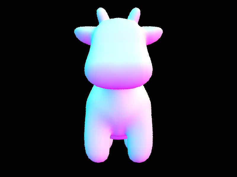
Comparison of Rendering Times
Below are a comparison of rendering times with and without BVH.
Cow without BVH: 41.2381s
Cow with BVH: 0.2033s
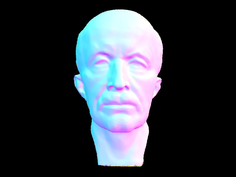
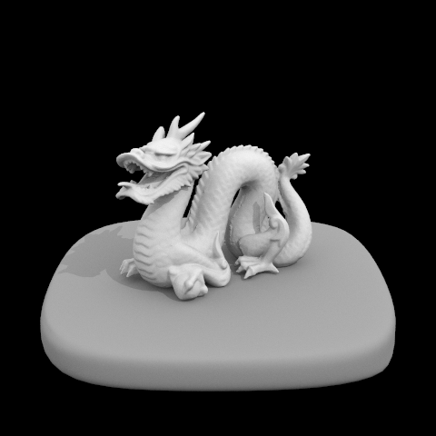
MaxPlanck with BVH: 0.2208s
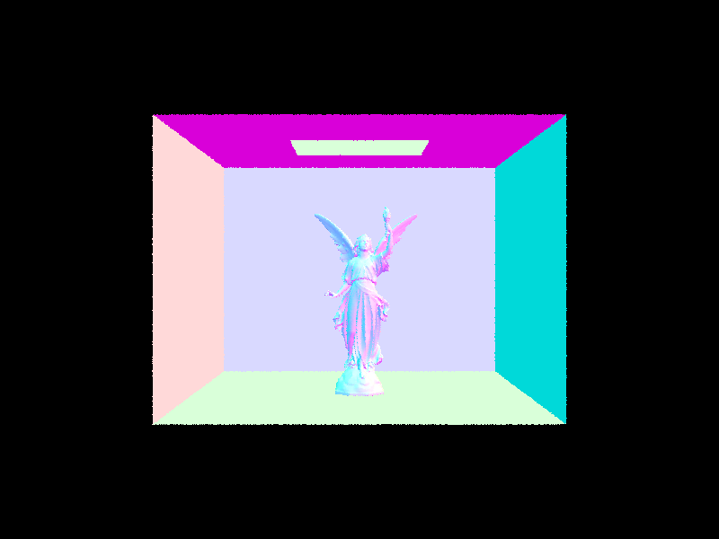
CBLucy with BVH: 0.1734s.
The cow renders much faster with BVH!. For MaxPlanck and CBLucy, I could not render them locally
without my computer almost crashing without BVH, so there is a very high improvement in efficiency
with BVH. This makes sense because instead of a ray checking that it intersects with thousands of primitive triangles,
it only has to check a few hundred bounding boxes first before checking directly against individual triangles.
It also allows me to preemptively reject rays that would never intersect certain primitives if the ray
misses the entire bounding box containing multipl primitives.
Section II: Illumination
Part 3: Direct Illumination
Task 3: Direct Lighting with Uniform Hemisphere Sampling
In this type of direct sampling method, I sampled from a uniform hemisphere up to a given number of samples. The probability distribution function of a uniform hemisphere is PDF = 1 / (2 * pi). To solve an estimation of the reflection equation, I found the BSDF of an object and a cos_theta value of incoming direction wi to a surface's normal in the object space. I then traced a new ray from an object towards hit_p, which is the hit point of the ray to the hemisphere, and the wi in world space, updating its min t value to EPS_F for some small error, and checked its intersections. If this new ray has no intersection with the scene, or cos_theta < 0, then this ray would not be added to the L_out value. Else, I populated a new intersection object with this intersection. If this ray intersected a light, I can retrieve its emissive value. Then, I added these values to L_out for the estimate by calculating f * L_in * cos / pdf. Once all the samples are traced, I normalized L_out by the number of samples. L_out now includes the zero and one bounce illumination.
Task 4: Direct Lighting by Importance Sampling Lights
In this type of direct sampling method, I sampled each of the lights in the scene rather than uniformly from a hemisphere. This reduces some noise and time. For each light, if the light is a point light, then I sampled the light only once for its BSDF and calculated cos_theta in object space, as sample_L only outputs in world space. I then generated a new ray, set its min and max to EPS_F and distToLight - EPS_F respectively, and checked for cos < 0 and if the new ray is a shadow ray. If either are true, then this ray would not be added to the L_out value. Else, I added to the L_out for point lights, with the same calculation for the estimated reflection equation. If the light is not a point light then I sampled it up to ns_area_light times and performed the same calculations as above. L_out now includes the zero and one bounce illumination.Comparison of Direct Sampling Methods at 64 Samples Per pixel
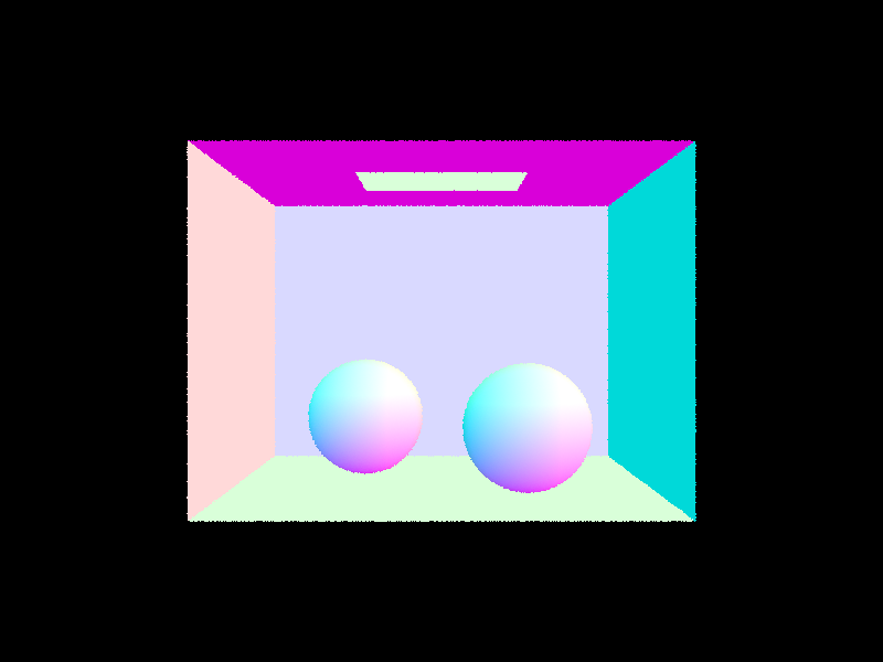
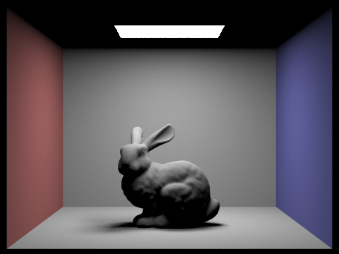
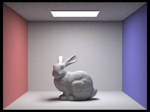
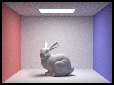
The most obvious effect of lighting / importance sampling is that the renders are much less noisy. This is because these lights are sampled directly and thus don't have extraneous rays that contribute little or not at all to the rendered image. The below images compare the bunny with just 16 rays per pixel and 8 samples per area light. The speed up of using importance sampling is fairly noteable because rays that would never otherwise reach the light are not accounted for by the sampling method. Of course, using more samples per pixel improves the quality and reduces noise for renders in either sampling method, although importance sampling converges to the correct output faster than uniform hemisphere sampling.
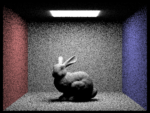

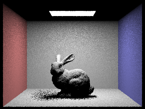
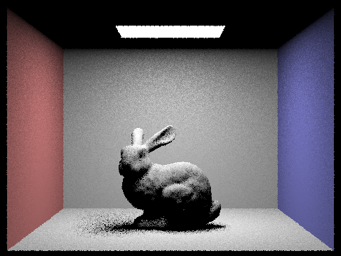
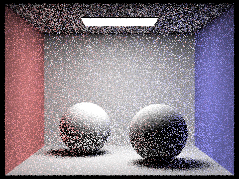
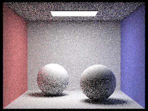
Comparison of Noise Levels with Different Light Ray Numbers
- 0.3717s
- 0.9353s
- 2.2761s
- 7.9116s
Notice how some of the noise especially around the bunny's shadow reduces with higher numbers of samples per area light. Even for a low number of samples per pixel, a high number of light rays can also converge to the correct output and reduce noise.


Part 4: Global Illumination
To implement indirect lighting, I needed to recursively call the at_least_one_bounce_radiance function on new rays and isect structs with the previous bounce's information, subject to termination via Russian Roulette. To achieve this, I set a continuation probability of 0.65 of performing another bounce to prevent infinite bounces, and set the first ray to max_ray_depth. I initialized L_out with once bounce of light from the given ray and isect. Then I used sample_f with the current wo value to calculated BSDF of (wo, *wi) and pdf of a diffuse lambertian BSDF to get L_in. From here I can generate my new ray and decrement its depth value by 1. I checked if the depth value is 0, if the ray does not intersect any bounding boxes, or if the Russian Roulette fails. If any of these are true, then I immediately terminate the ray's recursion. Otherwise, I can proceed to calculate for an intersection of the ray with the bounding box, calculate cos_theta, and recursively add to L_out with another call to at_least_one_bounce_radiance, normalized by the pdf and the continuation probability. The resulting L_out value is my final L_out, including all direct and indirect lighting.
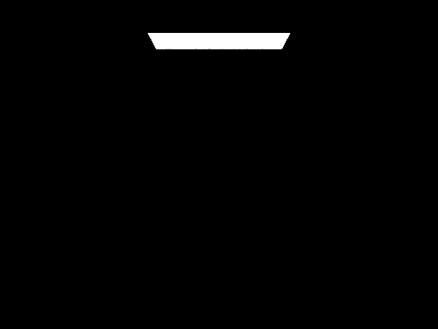
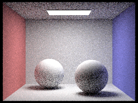
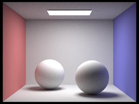
Comparison of Direct and Indirect at 64 Samples Per Pixel
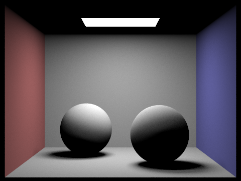
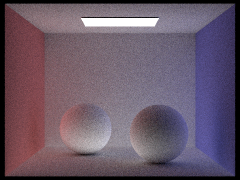
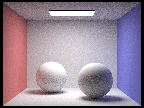
Comparison of Different Max Ray Depths at 64 Samples Per Pixel


Comparison of Different Sample Per Pixel Rates, 4 Light Rays, and Ray Depth 3


Part 5: Adaptive Sampling
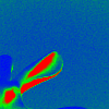
To implement adaptive sampling, I modified raytrace_pixel to check the convergence value of a pixel every 32 samples out of the maximum number of samples ns_aa, terminating once the convergence value is less than or equal to maxTolerance * mu, where convergence value I is based on a defaultly 95% confidence interval of having an average illuminance between mu - I and mu + I. For every sample, I collected its illuminance value x_k and added it into the summations s1 and s2. Every 32 samples out of the total number of samples, I calculated mu = s1 / n, sigma = sqrt((1 / (n - 1)) * (s2 - (s1^2) / n)), and I = 1.96 * (sigma / sqrt(n)). If it has converged, then I break the loop and set n as the number of samples for this pixel, and update the relevant buffers for this pixel.
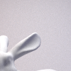
Below, I outputted a 100 x 100px square of the bunny at the given max samples per pixel of 2048 to get an accurate sample rate image. I tried rendering the bunny with smaller max sample rates, but it changed the sample rate image significantly enough I felt it wasn't useful to upload the full 480 x 360px image if it was not at 2048 samples per pixel. I hope this is enough to get a sense of how my adaptive sampling works for the bunny.
2048 samples per pixel, 1 sample per light, 5 max ray depth.