Rasterizer

Section I: Rasterization

Part 1: Rasterizing single-color triangles

To rasterize triangles, I first checked for if the centers of pixels are within the edges of the given triangles. To speed up the process of checking each pixel, I limited the search area to the bounding box of the triangle, clamped to the edges of the window (width x height). I checked the center of each pixel (x, y) by checking if the sample (x + 0.5, y + 0.5) is within the triangle's edges using the "Three Line Test" for a sample inside or on an edge, while also accounting for winding order. This test uses the normals of each edge and performs a dot product with a vector to measure the magnitude of a vector projection. If the sample is inside or on an edge, then I drew its associated pixel to the screen with the given color (RGB) values.

My algorithm is no worse than one that checks the each sample within the bounding box of the triangle because it only searches through pixels within this box or the window edges, and does not check any samples outside of this box. My algorithm then exhaustively searches each individual sample within this box.

Part 2: Antialiasing triangles

To add supersampling to my rasterization algorithm, I first used the sample rate to find the number of subdivisons per side (i.e. sample rate 16 is subdivided into a 4x4 grid), and then calculated the offset to find the center of each supersample by calculating 0.5 * (1/sqrt(sample_rate)). Then, for each pixel within the bounding box, I calculated the center of each supersample in coordinate space by using this offset and the index of the supersample. This new coordinate is then checked for membership in the triangle, and if the supersample is inside the triangle, I then added the supersample's color to the supersample buffer.

The supersample buffer is a vector of colors, with size width x height x sample_rate, and for a specific subpixel (x, y, i), it is located at (y * width + x) * sample_rate + s in the buffer.

To finally fill the target framebuffer with colors created from the supersamples, I first pulled the appropriate supersamples per pixel from the supersample buffer and averaged their colors. So for example for a sample rate of 4, I pulled the 4 supersamples corresponding to the same (x, y) pixel and averaged the four colors to get one RGB value which will be drawn to the screen.

Supersampling is useful because it helps antialias the edges of the triangles that we are rasterizing, as well as properly account for overlapping colors which may affect the same (x, y) pixel. Modifications made aside from expanding upon the intial rasterization algorithm was support for the supersample buffer, which had to properly be resized or cleared alongside the framebuffer target. I also had to use functions like resolve_to_framebuffer and fill_supersample to properly store and calculate averaged colors. However, the downside of supersampling is that requires much more computation time than simple sampling.

I used supersampling to antialias my triangles because the supersampling process makes edges appear "softer" by averaging the color values along the edges of the triangles by breaking up each pixel into multiple supersamples and evenly weighing each supersample's color.

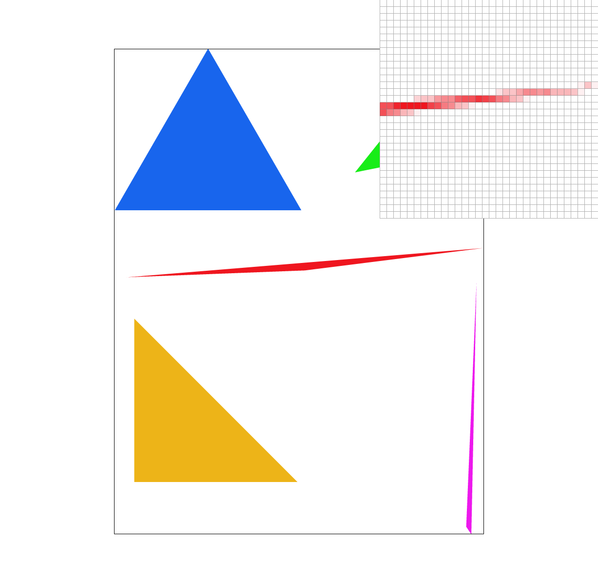
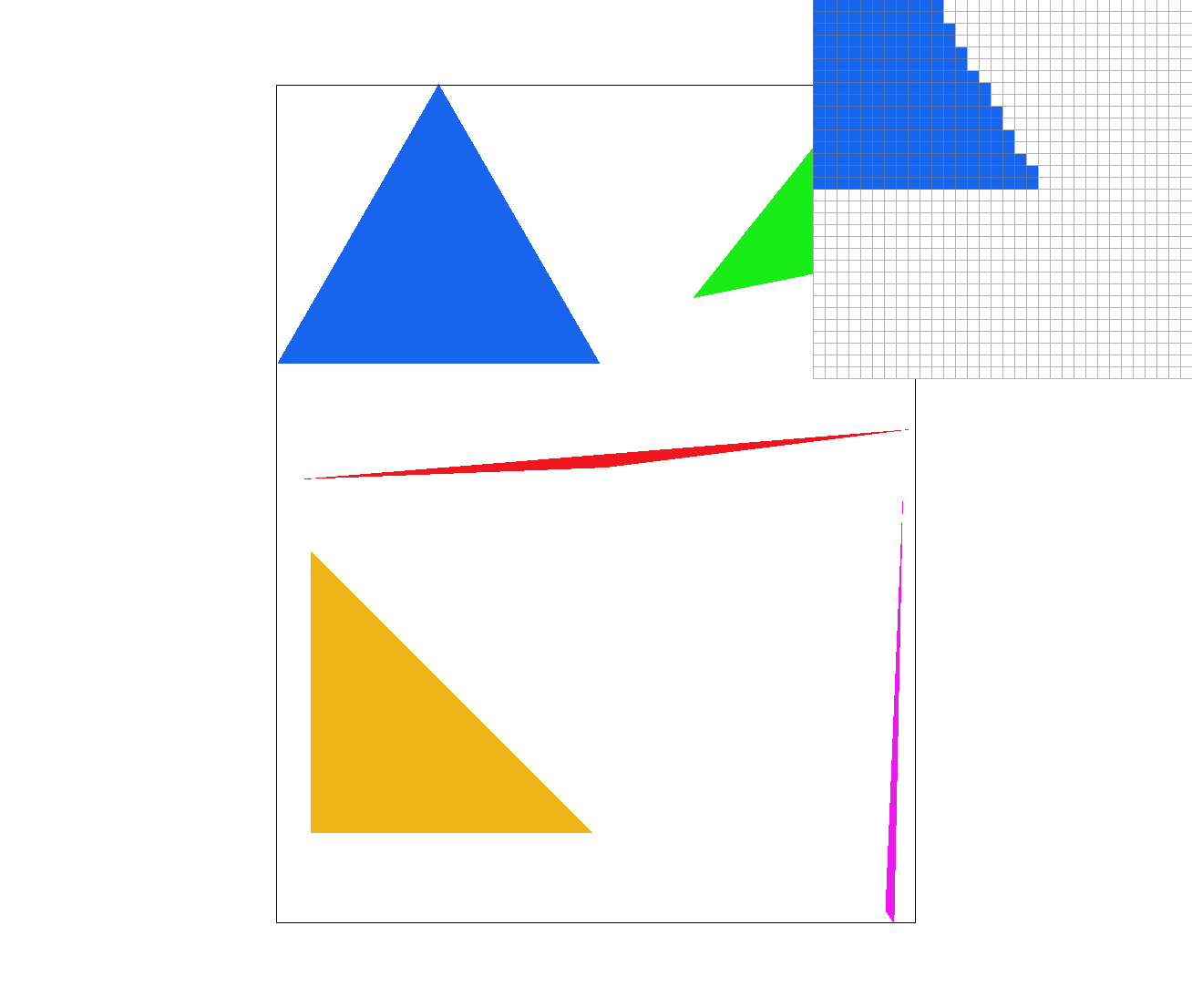
We can observe antialiasing along this far corner of the red triangle. As the sample rate goes up, each pixel has an increasing number of subpixels to sample from. As there are more supersamples, the quality of the antialiasing goes up because each pixel has more supersample coordinates to check and colors to average together. Antialiasing at the corners are more likely to have some supersamples inside and outside the triangle edges, so as there are more supersamples the corners will appear smoother because the colors will change more gradually.

Part 3: Transforms

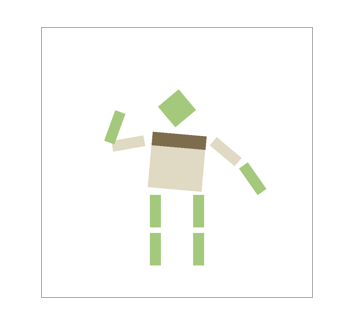
For colors and clothing, I thought it'd be fun to roughly depict Shrek. :)
I transformed the positions and rotations of his torso, head, and arms to make him seem as if he is waving or shaking his fist, as well as added an extra brown rectangle for his vest.

Section II: Sampling

Part 4: Barycentric coordinates

Barycentric coordinates are a way of representing coordinates as weighted averages of vertices. The corresponding weights, alpha, beta, and gamma, can be used to create a weighted average of colors or texture maps with UV values, so (x, y) near one of the vertices will have a high associated vertex weight and will have a stronger influenced color from that vertex. If (x, y) is at the center of mass / balance point of the triangle, where the weight distribution is equal, the color at (x, y) will be an even mix of all 3 vertex colors, as each color will be weighed evenly by 1/3rd.

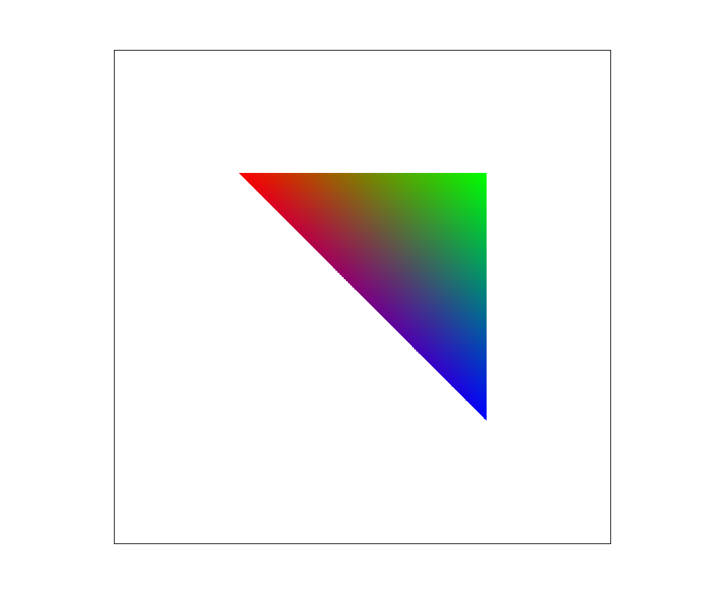
For example in this image, there is a green, blue, and red vertex. These colors spread out evenly from their respective vertices, and the center point is a neutral grey-ish color as it is equally influenced by all 3 colors. At some boundaries, you can notice colors mixing, such as brown near the red / green boundary, and purple at the blue / red boundry, because these points are mixing the two strongest color weights together.

Part 5: "Pixel sampling" for texture mapping

Pixel sampling uses barycentric coordinates to convert (x, y) coordinates from screen space to UV space and then to texel space. Converting from screen space to UV requires calculating barycentric coordinates to weigh the color values of the given UVs, and since these UV values are from [0, 1], I scaled U by the mipmap's width, and scaled V by the mipmap's height, based on the level passed into the sampling function. To prevent some bugs from occuring when zooming in / out of the image, I had to clamp the texel coordinates from 0 to one less than the mipmap's width and height. Based on the pixel sampling method, I then found the appropriate texture color to draw to the screen.

Nearest-pixel sampling: In this pixel sampling method, the returned color for a pixel is from the color of the "closest" pixel in the texture space. Visually, this appears as individual texture "pixels" scaling proportionally up when zoomed in, or vice versa. To find a corresponding texel value, I floored the value of the texel coordinates and returned the the color from that texel. Because nearest-pixel doesn't average any colors, it appears fairly blocky.

Bilinear sampling: Bilinear sampling uses bilinear filtering to linearly interpolate colors between nearby texels. The lerp function calculates a weighted average of colors from the four surrounding pixels in the horizontal direction, and then lerps these two values in the vertical direction. This filtering process returns colors that will improve anti-aliasing on the image due to this averaging process.

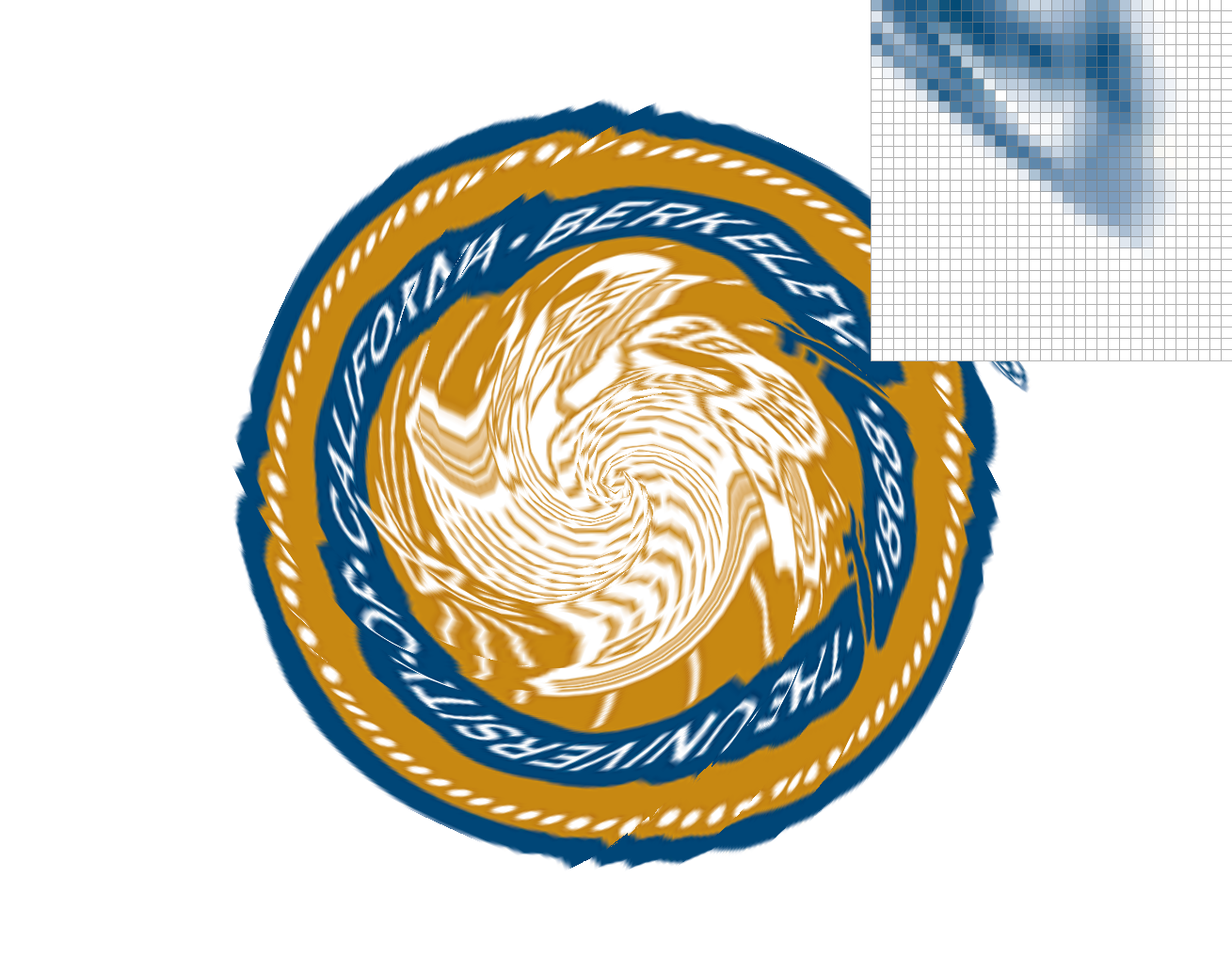
Nearest pixel sampling is clearly much more blocky and has more jaggies than bilinear pixel sampling at all sample rates. The trademark symbol in bilinear pixel sampling appears more smudged, and the edges of the seal are more anti-aliased. Increasing sample rate on nearest pixel sampling only blurs the jaggies, rather than smooth out the colors. Increasing sample rate on bilinear pixel sampling further smooths the changes in colors, though it is somewhat difficult to notice on the PNG above.

Part 6: "Level sampling" with mipmaps for texture mapping

To implement level sampling, I used the UV values passed into texture functions from the SampleParams struct, in order to calculate mipmap level D. Mipmap levels are used to work with texture magnification or minification, and applies different resolutions of the texture based upon the zoom of the image. Level 0 is the original high quality texture, and higher levels are more blurred. These levels are calculated based on the derivatives of UV colors passed by the rasterize function, and then adjusted based on the level sampling method. For nearest level sampling, the level returned from the level D computation is rounded to the nearest level. For bilinear level sampling, the level returned is then floored and ceiled to get level D and D+1, as well as a weight value from [0, 1]. This weight is then passed into the lerp function from before to calculate a weighted average of mipmap levels.

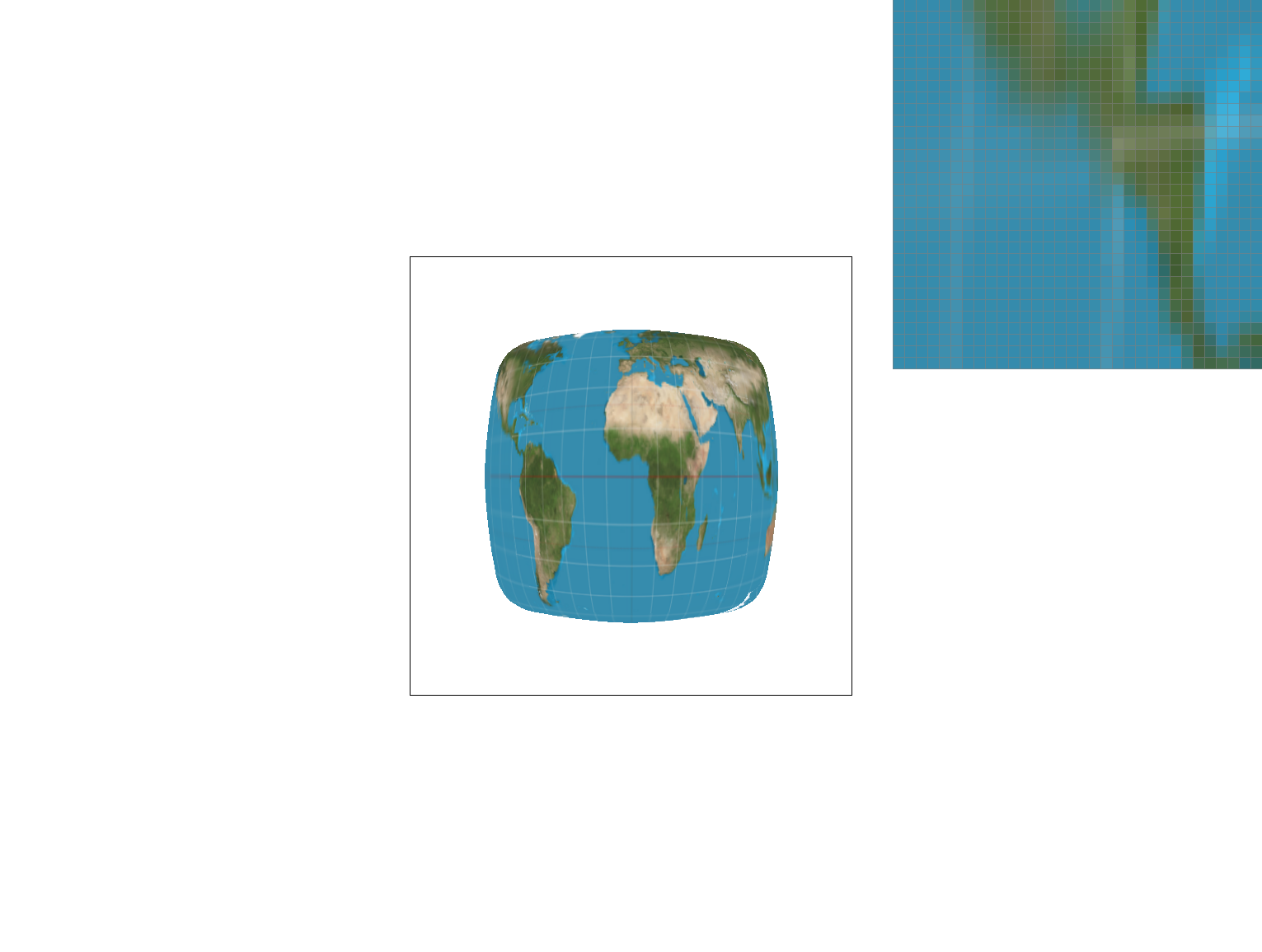
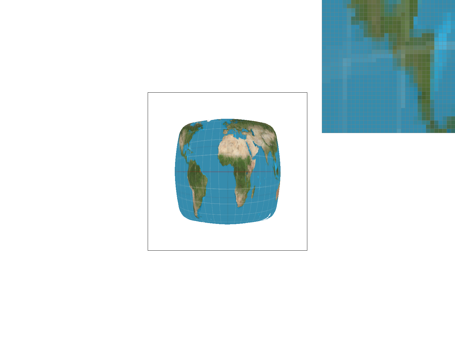
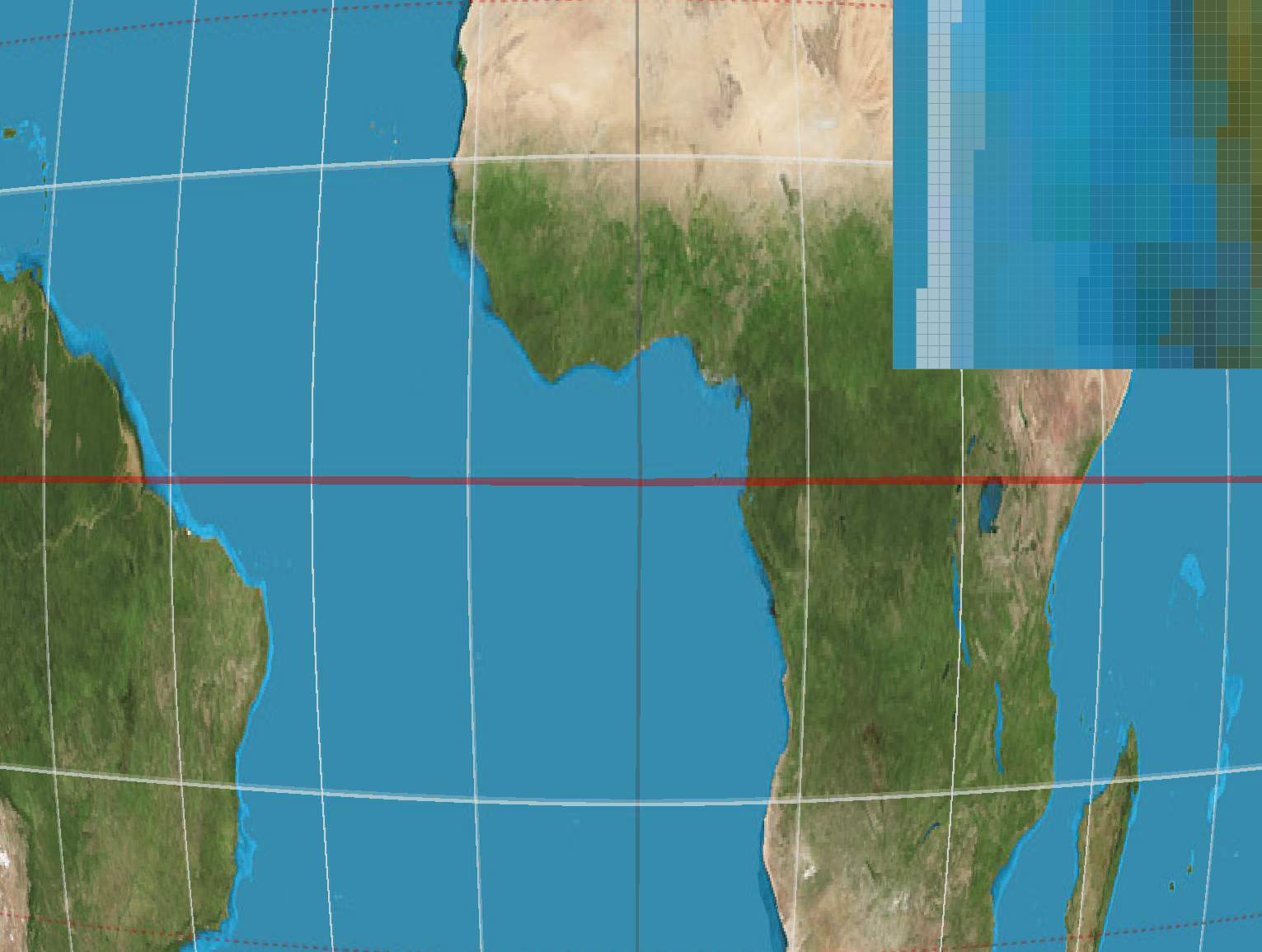
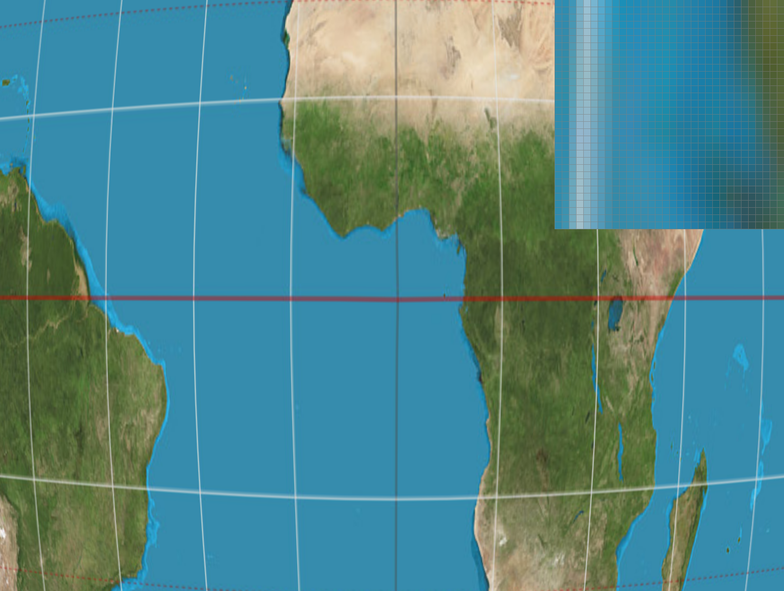
Zoomed out, it is clear that bilinear pixel and level sampling always adds more anti-aliasing than nearest pixel or level sampling. The longitude and latitude lines are much softer on nearest level and bilinear level sampling, and are blurred by bilinear pixel sampling. The colors of the land also become more uniform as the sampling methods change.

When zooming in, the difference between zero, nearest, and bilinear level sampling methods had little to no effect on the quality of the image, rather only the two pixel sampling methods made a difference. Zoomed out, the level sampling methods have more of an effect on the alising of the image.

The speed at which the images load is slower when zoomed in than when zoomed out at all pixel and sample levels. The antialiasing power of level sampling decreases as images are zoomed further in. The antialiasing power of pixel sampling appears about the same at different zoom levels, although when zoomed out there are less pixels representing elements like the longitude and latittude lines, so bilinear pixel sampling will anti-alias to smooth out some of the gaps in the pixels.

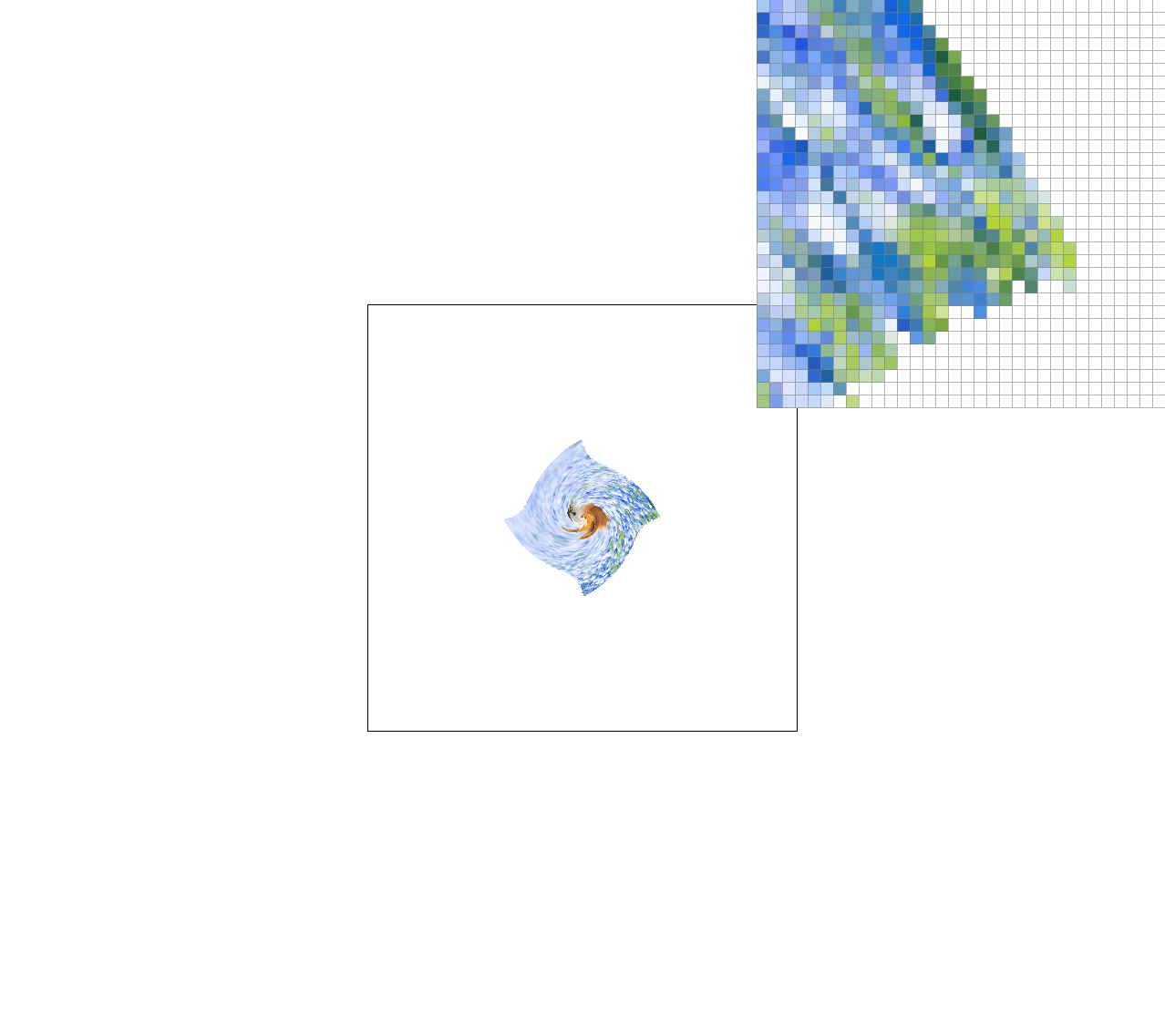
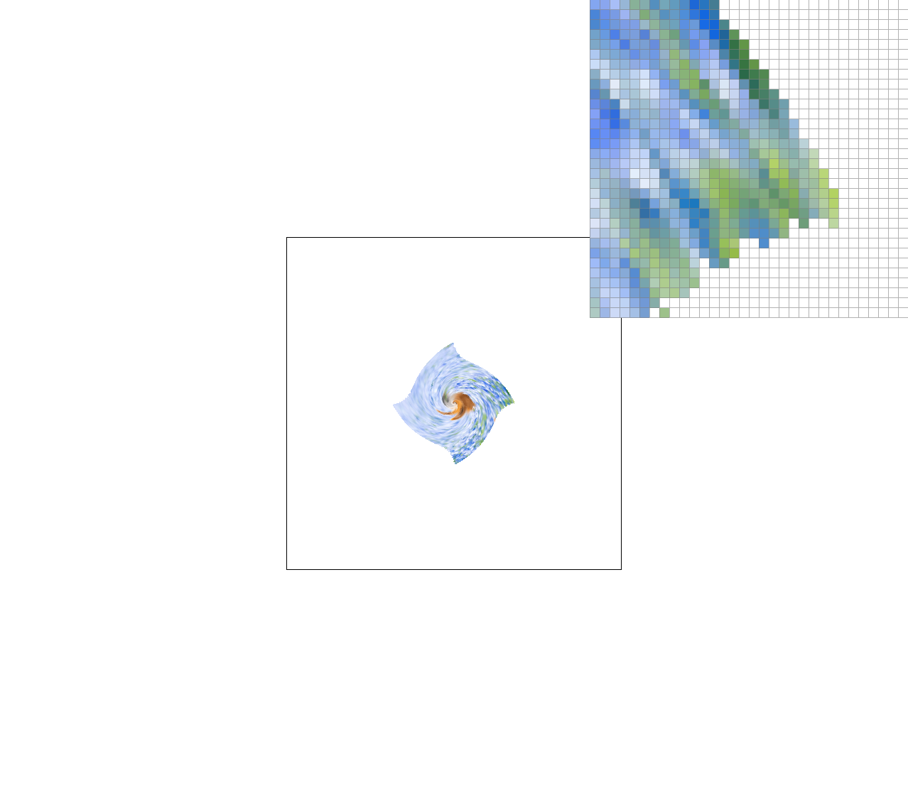
Below, I used the warped texture that originally had the Cal seal and replaced it with an image of a shiba inu in a meadow. The below show the differences at the corner at lsm = zero, lsm = nearest, psm = nearest, and psm = bilinear.