Pathtracer II

Implements the BSDF for special materials and calculates surface normals and reflective / refractive properties. Illuminates these materials with the previous part's ray tracer.

Part 1: Mirror and Glass Materials

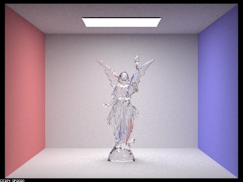
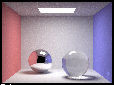
Mirror and glass materials with 256 samples/pixel, 4 samples/light, max depth 7.

Summary of Mirror Material Implementation

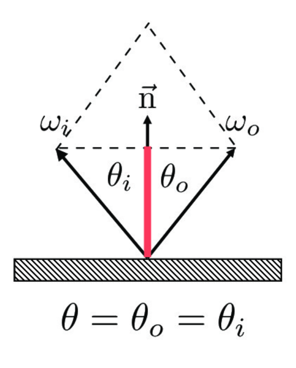
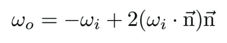
Mirror materials, or perfectly specular materials, depend on reflecting rays off a surface. I first implemented the basic reflection equation, where the surface normal in object space is (0, 0, 1). Since perfect specular surfaces reflect incoming rays at the same angle from the normal in the outgoing direction, I can use the following derived equation to calculate the reflected direction of a ray.

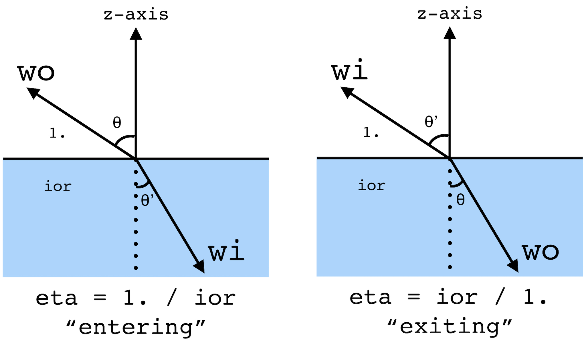
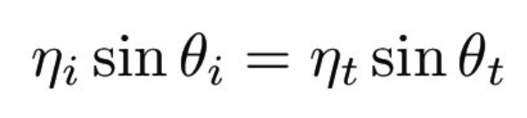
Summary of Glass Material Implementation

Glass or transparent materials depend on refracting rays as they pass from one volume to another. Refraction involves Snell's Law, which depends on the index of refraction (η) for the incident and exiting rays, which for this part is air to glass or glass to air. Air has a IOR of 1.00029, and glass has an IOR of 1.5-1.6, which I set to 1.55 in my renders. These indices affect how strongly a ray is refracted as it passes between two volumes. I needed to also take into account any total internal reflection that may occur from certain ray angles, that is when 1 - η^2(1 - cosθ^2) < 0, which means a ray did not successfully refract out of a volume. To approximate the physics of both refraction and reflection occuring, I used Schlick's approximation using reflection coefficient R to select whether or not a single ray reflects or refracts.

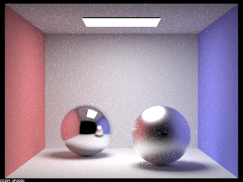
Below are comparisons of the mirror and glass spheres at different max ray depths, 64 samples/pixel and 4 samples/light.

Spheres depth 0.

Spheres depth 1.

Spheres depth 2.

Spheres depth 3.

Spheres depth 4.

Spheres depth 5.

Spheres depth 1000.

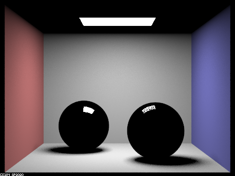
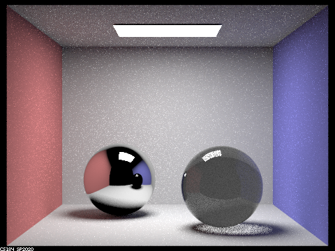
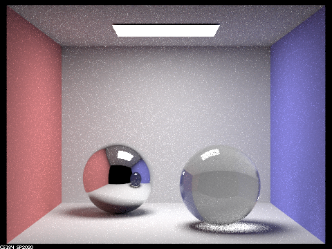
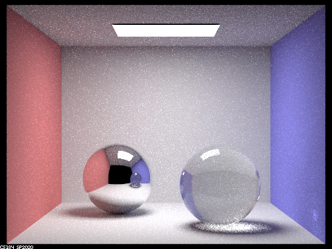
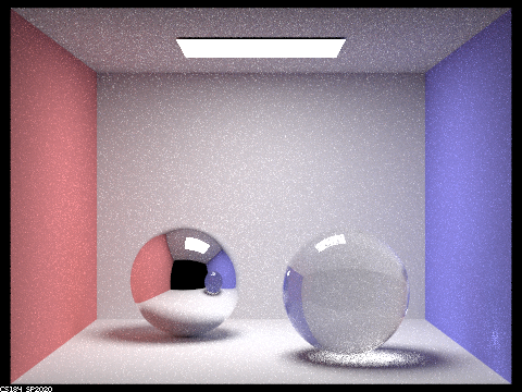
In the big picture, higher ray depths reflect and refract more of the wall's colors on the surfaces of the spheres as well as reflecting some rays onto the walls themselves. Max ray depth 0 is only the light from the ceiling, which is an emissive surface. Max ray depth 1 is a single bounce directly from the ceiling light off surfaces in the Cornell box, including the walls and the reflection of the light on the spheres. Max ray depth 2 is when the properties of specular and refractive surfaces begin to appear. The mirror sphere now reflects its surroundings on its surface, although the reflection of the glass ball on the mirror ball is black because the glass only reflects light off its surface at bounces 3 or higher. The glass sphere refracts rays directly from the light (as seen by the light shadow) but it has yet to refract indirect rays. Max depth 3 is when the scene begins to look more like the true result, but it is still missing some indirect rays. The mirror sphere's shadow now reflects some colors from the ground, and the mirror sphere now reflects the blue wall. Max depth 4 shows something interesting: a patch of light on the blue wall that represents rays that have exited the glass, as well as some reflection of the refracted light from the ground on the bottom of the sphere. And finally between max depth 5 and 100, you can see the reflection of the walls' colors on the surfaces and shadows of both spheres, as well as some indirect brights spots in the glass sphere's shadow and the blue wall.

Part 2: Microfacet Materials

Summary of Microfacet Material Implementation

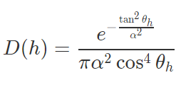
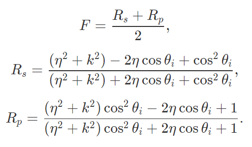
To implement microfacet materials, I need to calculate the microfacet BRDF, which depends on F: the Fresnel term, G: the shadowing-masking term, D: the normal distribution function (NDF), n: the macro surface normal, and h: the half vector between the incoming and outgoing rays.

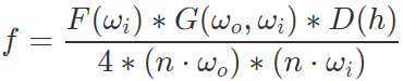
I implemented the following two variables for the microfacet BRDF:
D(h), the normal distribution function for a half vector h, depends on α, which defines how specular / diffuse the surface of the material is. A high α value has a rough macro surface, which will cause the surface normals to be more offset and scattering rays in a diffuse manner. A rough surface results in a half-angle vector that is offset from the surface normal.

F(wi), the Fresnel term of the incoming ray for air-conductor surfaces, I calculated the following approximation, for the given eta and k indices of refraction.

Now that the microfacet BRDF is implemented, I can properly represent microfacet materials at different alpha values. Unfortunately, renders of these materials are very noisy with cosine hemisphere sampling and require many samples to properly represent the shader's reflective properties. To remedy this problem, I implemented importance sampling according to the Beckmann NDF distribution. By sampling for θ and φ according to these two probably distribution functions, I can converge to a render that with fewer samples per pixel represents the reflective properties of a microfacet BRDF.

And then finally I can calculate the probability distribution function of sampling wi with respect to the solid angle rather than θ and φ.

Microfacet materials with 256 samples/pixel, 4 samples/light, max depth 7.

Dragon with α = 0.005.

Dragon with α = 0.05.

Dragon with α = 0.25.

Dragon with α = 0.5.

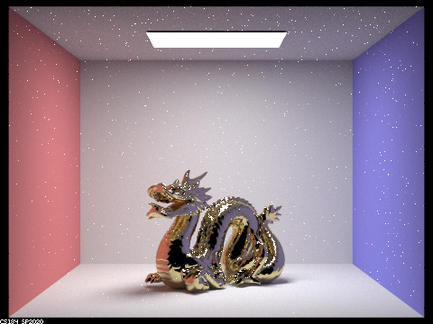
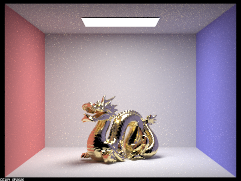
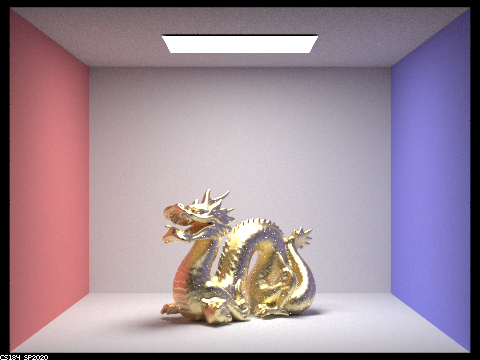
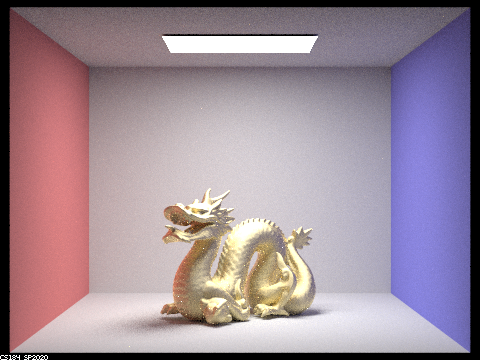
The larger the α value, the more diffuse the gold appears on the dragon. Lights and shadows are less stark and the surface appears less polished and softer. The base gold color is also more noticeable for high α values. When α is close to 0, the material becomes a perfect mirror and only reflects the colors of the surroundings rather than the color of the material itself. This is why the dragon with α = 0.005 appears dark and polished, because it is mostly directly reflecting the colors of the walls as well as the black area where the camera is located. It also has sharper reflections of light and shadows. At α = 0.5, the dragon has much softer reflective areas and takes on more of its yellow base color and less of the red and blue walls' colors.

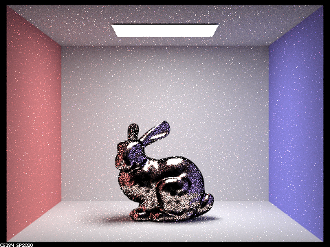
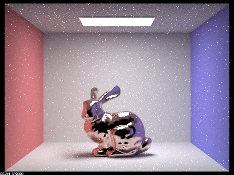
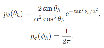
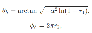
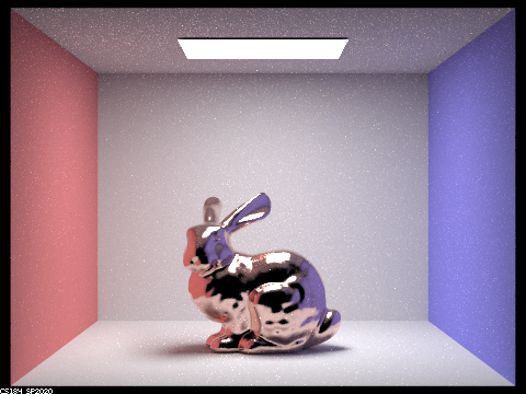
Bunny with cosine hemisphere sampling.

Bunny with importance sampling (Beckmann NDF).

With hemisphere sampling, the bunny's surface is much noisier and darker at the same number of samples as importance sampling. With higher samples, it converges closer to the appearance of importance sampling, but at the cost of computation. The copper colors of the bunny are much more apparent on the bunny with importance sampling, as evidenced by the reflection of the white walls in a rosy color off the bottom and top of the bunny.

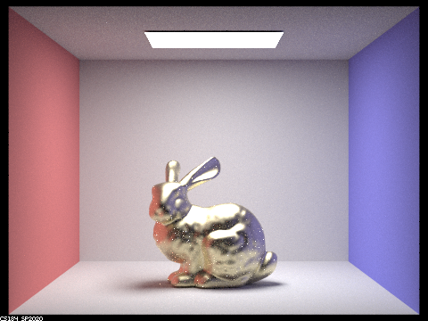
Bunny with the brass refractive index at α = 0.25.

Using the refractive index website, I applied the "brass" material to the Cornell Box bunny. Notice how with this new refractive index, the bunny is now reflecting the white walls as a yellow color rather than as pink.
α = 0.25
η = 0.45080 0.52920 0.93760
k = 3.3806 2.7553 1.9274